Post Zero: A Cascading Collection of Caveats

Here we make our introductions and discuss what these collections of posts might be

Last Updated: Monday, October 03, 2022 - 19:19:50.

A Brief Yet Accurate Summary:

Jason M. Osborne received a Ph.D in Mathematics from North Carolina State University in 2007. He has been a mathematics educator at several universities (currently Appalachian State) and has published a number of peer-reviewed articles for engineering and mathematics journals.

Caveat: Don’t worry, in general I will not be posting prints of full length mathematics articles. In most cases, I am much more interested in using imagery and animations to post about the “ideas” and “motivations” behind the scenes as shown in Figures 1 and 2.

$Effects of Curvature on Area. (top/left) This is a technical article wherein Differential Geometry is applied to a “chasing problem on a sphere”. I am proud of this article, but it was written for a specific audience that has the benefit of a background in Calculus and Differential Equations on and Differential Geometry of the sphere. An underlying idea behind this article is that a sphere has a quantifiable curvature. In future posts, I will try in my own way to illustrate (literally) curvatures manifestations on area. (middle) This figure shows that a 1 x 1 “square” on the sphere will generally have area not equal to 1, but as the radius $\rho$ of the sphere grows the area $A$ will get closer and closer to 1. (bottom/right) This figure shows that a 1 x 1 “square” on sphere changes with latitude and is distorted from 1. As this “square” approaches the equator the distortion in area becomes less but not zero (except at one point!). Compared to a 1 x 1 square on a flat sheet of paper which has area exactly equal to 1, the curvature of a 1 x 1 “square” on a sphere manifests as loss/gain in area. Computing the area $A$ on a surface like an $l \times w$ rectangle on a sphere of radius $\rho$ at latitude $m$ (for meridians) is possible by evaluating a (surface area) double integral which, in the case of a sphere, evaluates to the formula $A=\rho w\csc(m)\left(\cos(m)-\cos\left(\frac{l}{\rho}+m\right)\right)$. A future post will discuss the origins of this formula and justification of the observations above, which really needs to start with just what it means to be a 1 x 1 “square” on a sphere.$ $Effects of Curvature on Area. (top/left) This is a technical article wherein Differential Geometry is applied to a “chasing problem on a sphere”. I am proud of this article, but it was written for a specific audience that has the benefit of a background in Calculus and Differential Equations on and Differential Geometry of the sphere. An underlying idea behind this article is that a sphere has a quantifiable curvature. In future posts, I will try in my own way to illustrate (literally) curvatures manifestations on area. (middle) This figure shows that a 1 x 1 “square” on the sphere will generally have area not equal to 1, but as the radius $\rho$ of the sphere grows the area $A$ will get closer and closer to 1. (bottom/right) This figure shows that a 1 x 1 “square” on sphere changes with latitude and is distorted from 1. As this “square” approaches the equator the distortion in area becomes less but not zero (except at one point!). Compared to a 1 x 1 square on a flat sheet of paper which has area exactly equal to 1, the curvature of a 1 x 1 “square” on a sphere manifests as loss/gain in area. Computing the area $A$ on a surface like an $l \times w$ rectangle on a sphere of radius $\rho$ at latitude $m$ (for meridians) is possible by evaluating a (surface area) double integral which, in the case of a sphere, evaluates to the formula $A=\rho w\csc(m)\left(\cos(m)-\cos\left(\frac{l}{\rho}+m\right)\right)$. A future post will discuss the origins of this formula and justification of the observations above, which really needs to start with just what it means to be a 1 x 1 “square” on a sphere.$ $Effects of Curvature on Area. (top/left) This is a technical article wherein Differential Geometry is applied to a “chasing problem on a sphere”. I am proud of this article, but it was written for a specific audience that has the benefit of a background in Calculus and Differential Equations on and Differential Geometry of the sphere. An underlying idea behind this article is that a sphere has a quantifiable curvature. In future posts, I will try in my own way to illustrate (literally) curvatures manifestations on area. (middle) This figure shows that a 1 x 1 “square” on the sphere will generally have area not equal to 1, but as the radius $\rho$ of the sphere grows the area $A$ will get closer and closer to 1. (bottom/right) This figure shows that a 1 x 1 “square” on sphere changes with latitude and is distorted from 1. As this “square” approaches the equator the distortion in area becomes less but not zero (except at one point!). Compared to a 1 x 1 square on a flat sheet of paper which has area exactly equal to 1, the curvature of a 1 x 1 “square” on a sphere manifests as loss/gain in area. Computing the area $A$ on a surface like an $l \times w$ rectangle on a sphere of radius $\rho$ at latitude $m$ (for meridians) is possible by evaluating a (surface area) double integral which, in the case of a sphere, evaluates to the formula $A=\rho w\csc(m)\left(\cos(m)-\cos\left(\frac{l}{\rho}+m\right)\right)$. A future post will discuss the origins of this formula and justification of the observations above, which really needs to start with just what it means to be a 1 x 1 “square” on a sphere.$

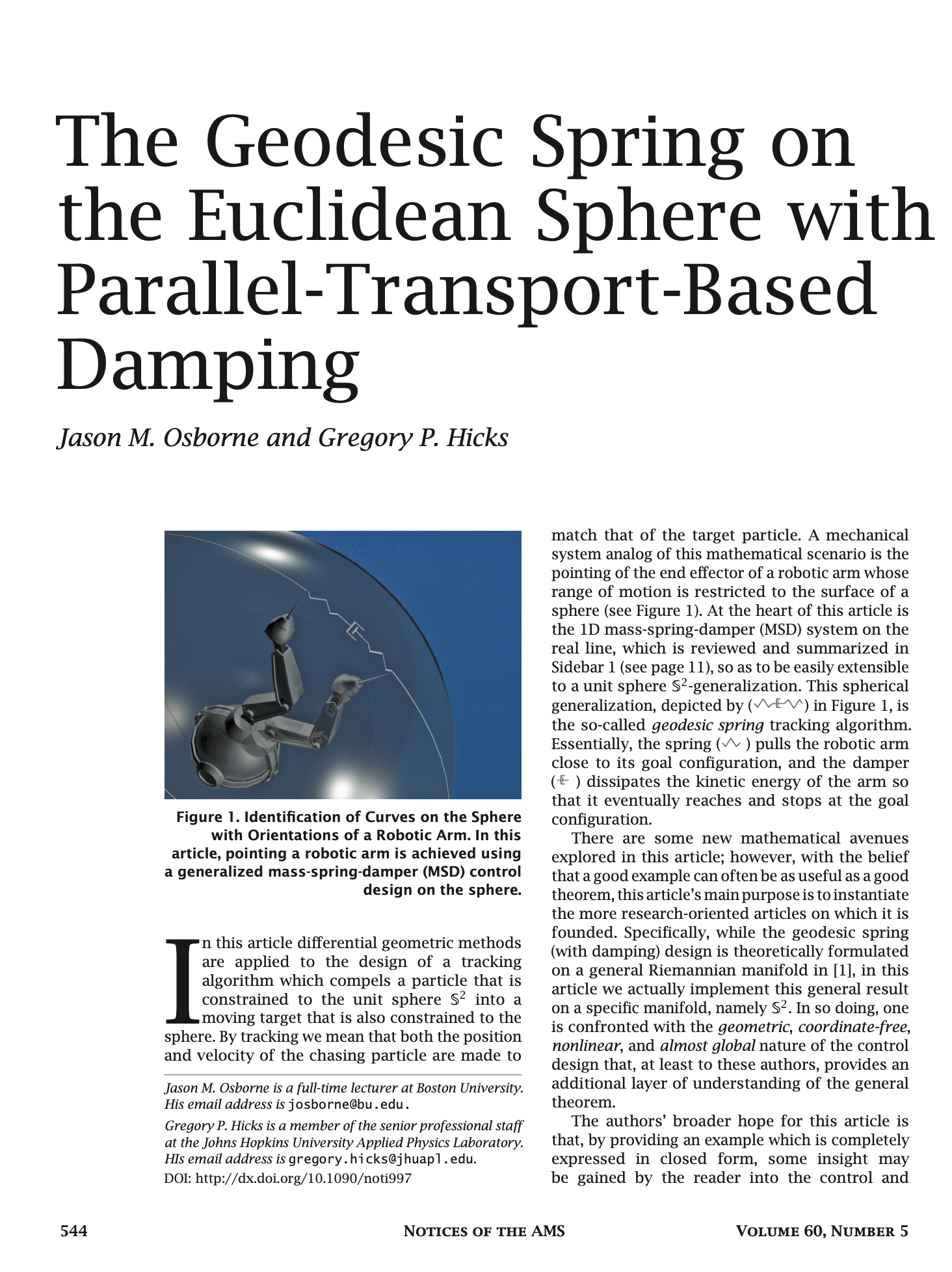
Figure 1: Effects of Curvature on Area. (top/left) This is a technical article wherein Differential Geometry is applied to a “chasing problem on a sphere”. I am proud of this article, but it was written for a specific audience that has the benefit of a background in Calculus and Differential Equations on and Differential Geometry of the sphere. An underlying idea behind this article is that a sphere has a quantifiable curvature. In future posts, I will try in my own way to illustrate (literally) curvatures manifestations on area. (middle) This figure shows that a 1 x 1 “square” on the sphere will generally have area not equal to 1, but as the radius $\rho$ of the sphere grows the area $A$ will get closer and closer to 1. (bottom/right) This figure shows that a 1 x 1 “square” on sphere changes with latitude and is distorted from 1. As this “square” approaches the equator the distortion in area becomes less but not zero (except at one point!). Compared to a 1 x 1 square on a flat sheet of paper which has area exactly equal to 1, the curvature of a 1 x 1 “square” on a sphere manifests as loss/gain in area. Computing the area $A$ on a surface like an $l \times w$ rectangle on a sphere of radius $\rho$ at latitude $m$ (for meridians) is possible by evaluating a (surface area) double integral which, in the case of a sphere, evaluates to the formula $A=\rho w\csc(m)\left(\cos(m)-\cos\left(\frac{l}{\rho}+m\right)\right)$. A future post will discuss the origins of this formula and justification of the observations above, which really needs to start with just what it means to be a 1 x 1 “square” on a sphere.

$Gauss Curvature Illustration. In a future post, I will try in my own way to illustrate (literally) how the mathematician Carl Friedrich Gauss (1827) used a ratio of areas to quantify the curvature of a surface at a point. Note that as an example, for the surface $f(x,y)=-x^2-y^2+3$ at the point $P=(1/2,-1/4)$, the ratio of pink area (on the surface) to black area (on the sphere) as shown approaches the number $0.793236$ which is close to $64/81 \approx .790123$. That is, the Gauss Curvature of this function at this point is about $0.79$.$ $Gauss Curvature Illustration. In a future post, I will try in my own way to illustrate (literally) how the mathematician Carl Friedrich Gauss (1827) used a ratio of areas to quantify the curvature of a surface at a point. Note that as an example, for the surface $f(x,y)=-x^2-y^2+3$ at the point $P=(1/2,-1/4)$, the ratio of pink area (on the surface) to black area (on the sphere) as shown approaches the number $0.793236$ which is close to $64/81 \approx .790123$. That is, the Gauss Curvature of this function at this point is about $0.79$.$

Figure 2: Gauss Curvature Illustration. In a future post, I will try in my own way to illustrate (literally) how the mathematician Carl Friedrich Gauss (1827) used a ratio of areas to quantify the curvature of a surface at a point. Note that as an example, for the surface $f(x,y)=-x^2-y^2+3$ at the point $P=(1/2,-1/4)$, the ratio of pink area (on the surface) to black area (on the sphere) as shown approaches the number $0.793236$ which is close to $64/81 \approx .790123$. That is, the Gauss Curvature of this function at this point is about $0.79$.

He is constantly amazed by how a few scribbles of mathematical symbology on a piece of paper can convey any meaning at all.

Caveat: Don’t worry, I am as annoyed as many of you with the sheer amount of symbology in mathematics in general and how this can obscure the ideas behind the symbols. Whenever possible (which honestly will be every chance I get), imagery will be over-used to motivate the ideas being discussed in posts. For example, when trying to learn about Differential Geometry from the web, it will be nearly impossible to avoid the language and symbology of Tensors. In a future post, as shown in Figure 3, I will try in my own way to illustrate (literally) Tensors as multi-dimensional information storage and show actual usage of Tensors via computation in the context of Curvature (from the perspective’s of both Riemann and Cartan)

On Tensors. (top/left) A Tensor as Written by Einstein in “Einstein’s 1912 Manuscript on the Special Theory of Relativity” (published by George Braziller Inc.) (middle) An Illustration of a Tensor as a System of Drawers Containing Stored Objects/Data (bottom/right) The Many, Many Ways to View the Data Stored in a Tensor

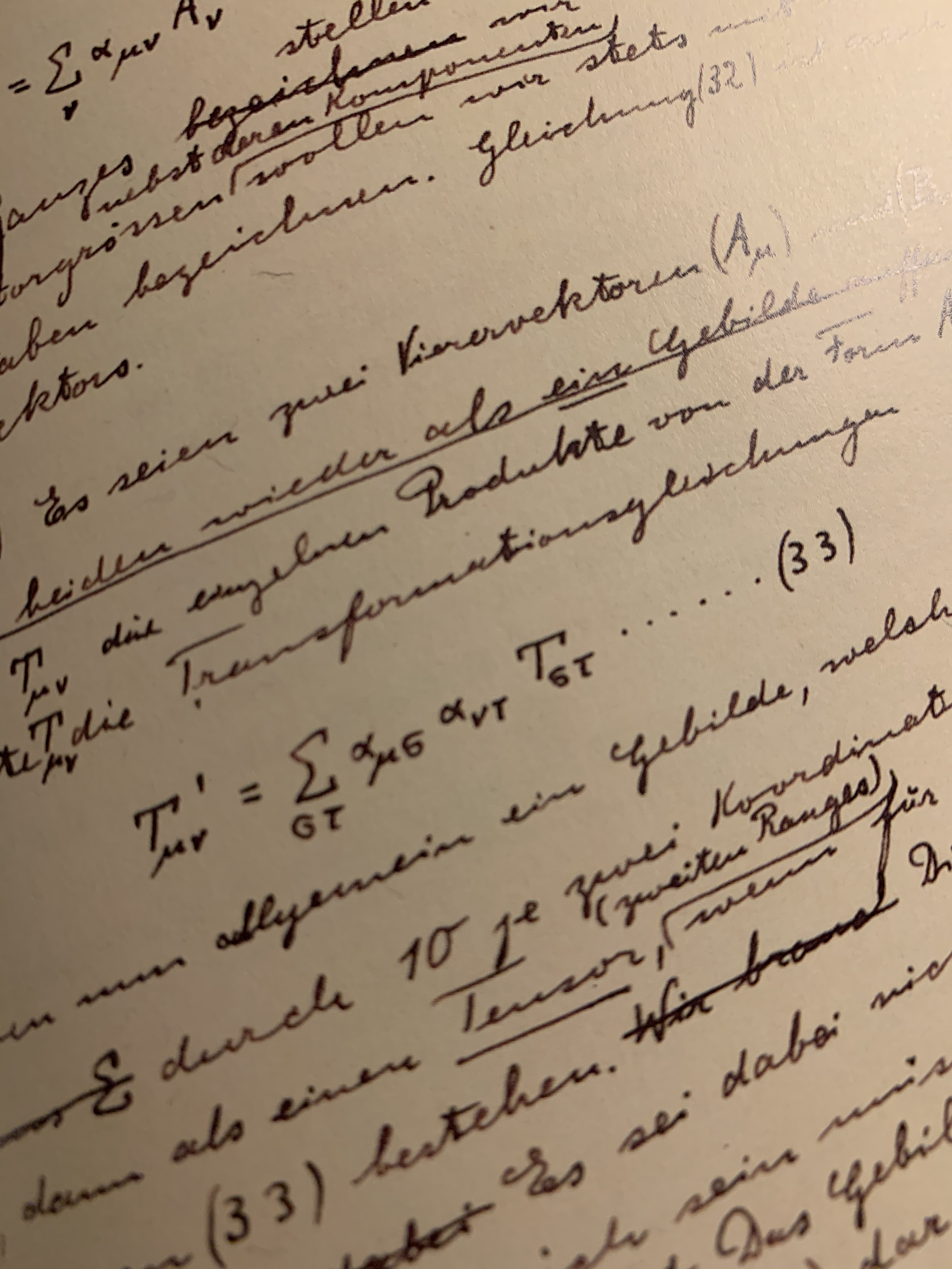
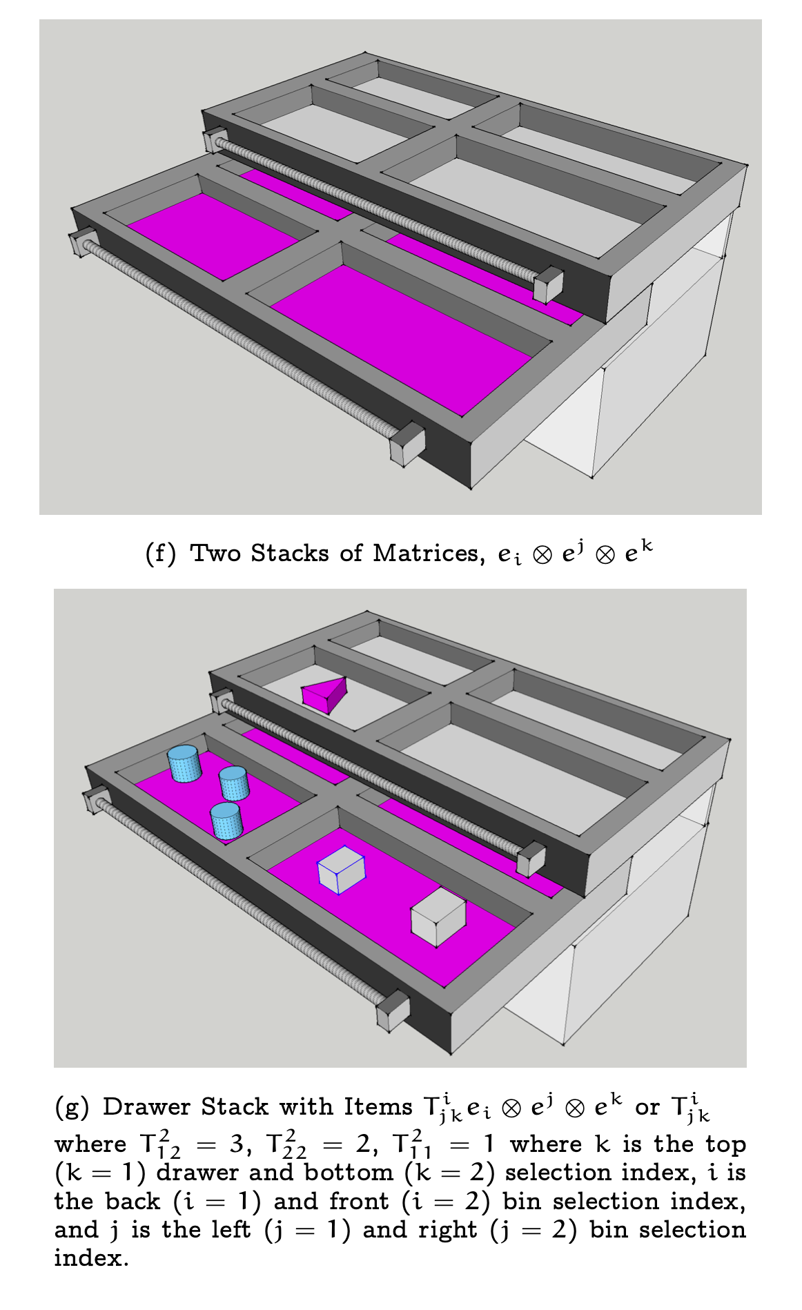
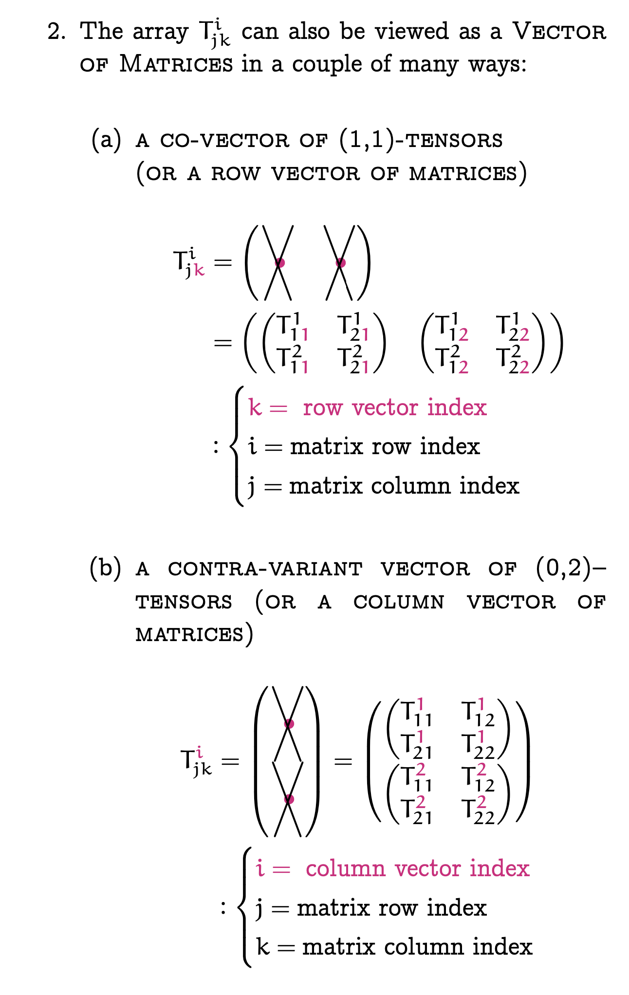
Figure 3: On Tensors. (top/left) A Tensor as Written by Einstein in “Einstein’s 1912 Manuscript on the Special Theory of Relativity” (published by George Braziller Inc.) (middle) An Illustration of a Tensor as a System of Drawers Containing Stored Objects/Data (bottom/right) The Many, Many Ways to View the Data Stored in a Tensor

When being a Mathematician proves too challenging he tries to think about the variety of ways he can make mathematics more widely accessible. For example, in his first book, a graphic novel, On Maps and Math and Making Friends: A Curvature Story, he artfully explains in nearly 100 full color, animated pages what can and has been written by others in a page or two of black & white, perfectly stationary mathematical formulas.

Caveat: Don’t worry, I wouldn’t ask you to invest time in this “Posts–Project” with me without giving you some more examples of what to expect in style and content of future posts. Some posts will be part of larger projects like books. In Figure 4 we can see some screenshots of the book “A Curvature Story” (See More Screenshots)

A Curvature Story Excerpts. (top/left) Meet Pete-A Character in the Story (middle) Math In Animated Graphic Novel Form (bottom/right) Math In Traditional Form: The Professor’s Indecipherable Notes

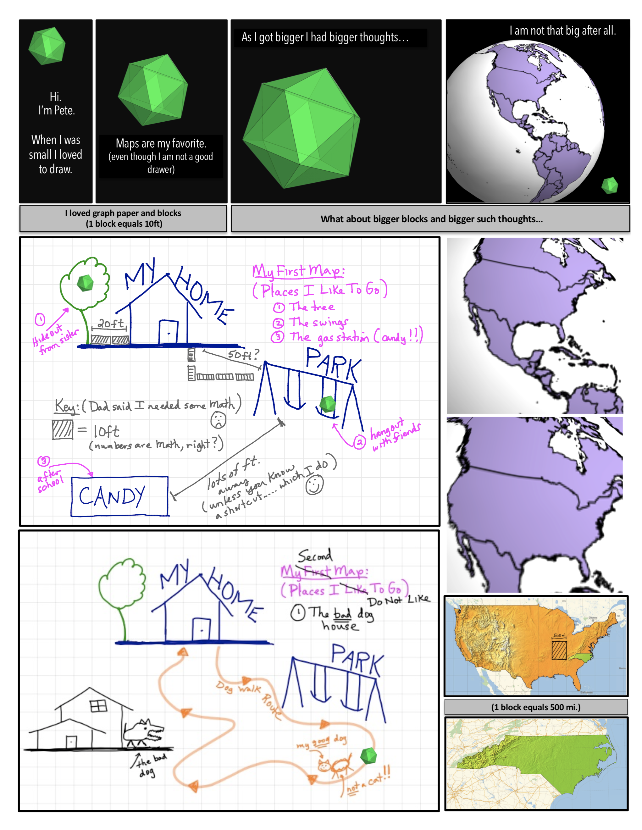
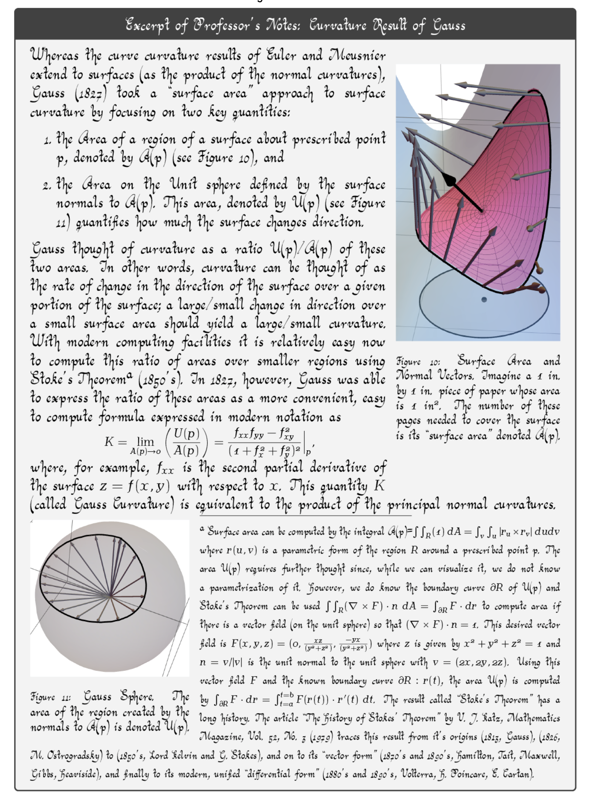
Figure 4: A Curvature Story Excerpts. (top/left) Meet Pete-A Character in the Story (middle) Math In Animated Graphic Novel Form (bottom/right) Math In Traditional Form: The Professor’s Indecipherable Notes

Figure 5: Get a “A Curvature Story” on Apple Books

He has never once been accused of being concise.

Caveat: Don’t worry, not concise equals more Posts in the future…

In The Future…these posts will likely focus on my interests in the tensor computations necessary to solve problems in Applied Differential Geometry. Posting will most likely occur when (1) I have spent a lot of time figuring something out and have the thought “Why didn’t someone explain it like that before?” I will try to show the lines of thought that most helped me come to my own understanding (2) I have finished a set of notes or a small book and want to give a short summary. (3) I get bogged down in too large a project and just want to make a post to feel like I have made progress.

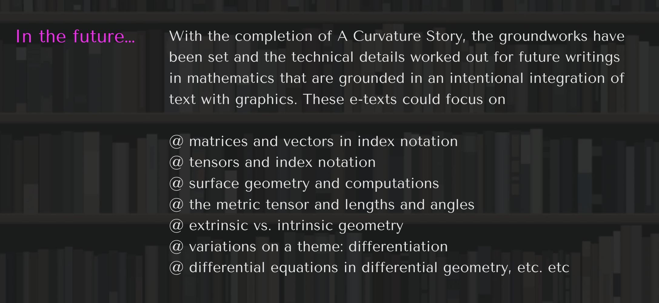
Figure 6: In The Future…these posts will likely focus on my interests in the tensor computations necessary to solve problems in Applied Differential Geometry. Posting will most likely occur when (1) I have spent a lot of time figuring something out and have the thought “Why didn’t someone explain it like that before?” I will try to show the lines of thought that most helped me come to my own understanding (2) I have finished a set of notes or a small book and want to give a short summary. (3) I get bogged down in too large a project and just want to make a post to feel like I have made progress.