The Cost Of Curvature
An attempt is made to re-cast the curvature of a sphere in terms of area (meters squared) and money (dollars). It turns out that the curvature of the earth doesn’t cost that much. Some of the mathematical ideas touched on in this post are surface area, arc-length, and great circles.
Last Updated: Monday, October 03, 2022 - 19:22:58.
In the animated graphic novel On Maps and Maths and Making Friends: A Curvature Story the concept behind and computation of curvature is visually and intuitively introduced for surfaces (of which the sphere is but one example). While giving a presentation about this book to the inviting folks at Science Cafe (video recording here), I received a question from one of member of the audience about an area result I was using to motivate curvature. Their question around about minute 26, which was essentially “How can it make sense to have a 1 x 1 square on the sphere?”, has stuck with me because of how I wished I had answered their question. This post is the not-so-concise answer I would like to have given.
Definitions: Meridians, Parallels, and Squares
Consider the images of the sphere shown in Figures 1, 2, and 3. When the sphere is viewed from the top, the Parallels are the circles (the rims of a wheel) and the Meridians are lines (the spokes of the wheel). More precisely, the Meridians are the circles of constant Longitude (i.e. the Lines of Longitude) while the Parallels are the circles of constant Latitude (i.e. the Lines of Latitude). Mathematically, we can describe a sphere of radius \(\rho\) parametrically as \[\begin{align} r(\theta,\phi)&=(\rho\sin(\phi)\cos(\theta),\rho\sin(\phi)\sin(\theta),\rho\cos(\phi)) \\ &= (f(\phi)\cos(\theta),f(\phi)\sin(\theta),h(\phi)), \end{align}\] where \[\begin{align} f(\phi)=\rho\sin(\phi)\;\; \mbox{and}\;\; h(\phi)=\rho\cos(\phi). \end{align}\] In this case, \(\theta^{R}\) is the angle (in radians) from the Prime Meridian to a Line of Longitude while the \(\phi^{R}\) is the angle (in radians) from the North Pole to a Line of Latitude. The value \(\psi^{\circ}=90^{\circ}-\phi^{\circ}\) is therefore the angle in degrees from the Equator to a Line of Latitude. The value \(\psi^{\circ}=90^{\circ}-\phi^{\circ}\) can also be called the \(\psi^{\circ}\)th Parallel.
Now define a Square on a Sphere to be the region between two equally spaced Latitudes and two Longitudes. The key to this definition is being able to correctly determine distances on a sphere.
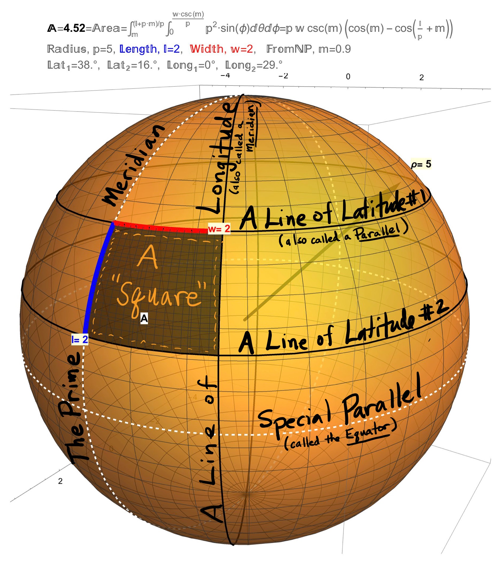
Figure 1: Special Curves and Regions On a Sphere: The Meridians are the circles of constant Longitude (i.e. the Lines of Longitude) while the Parallels are the circles of constant Latitude (i.e. the Lines of Latitude). Define a Square to be the region between two equally spaced Latitudes and two Longitudes.
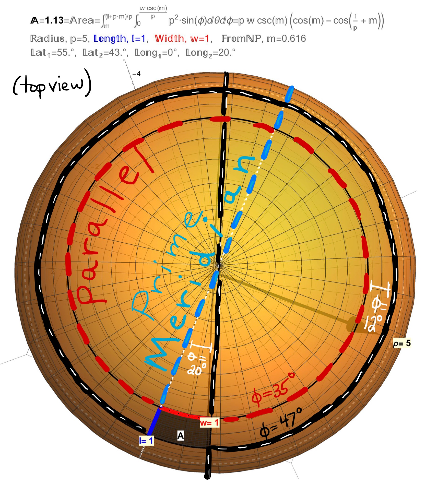
Figure 2: Special Curves and Regions On a Sphere: Viewing a sphere from the top, the Parallels are the circles (the rims of a wheel) and the Meridians are the lines (the spokes of the wheel).
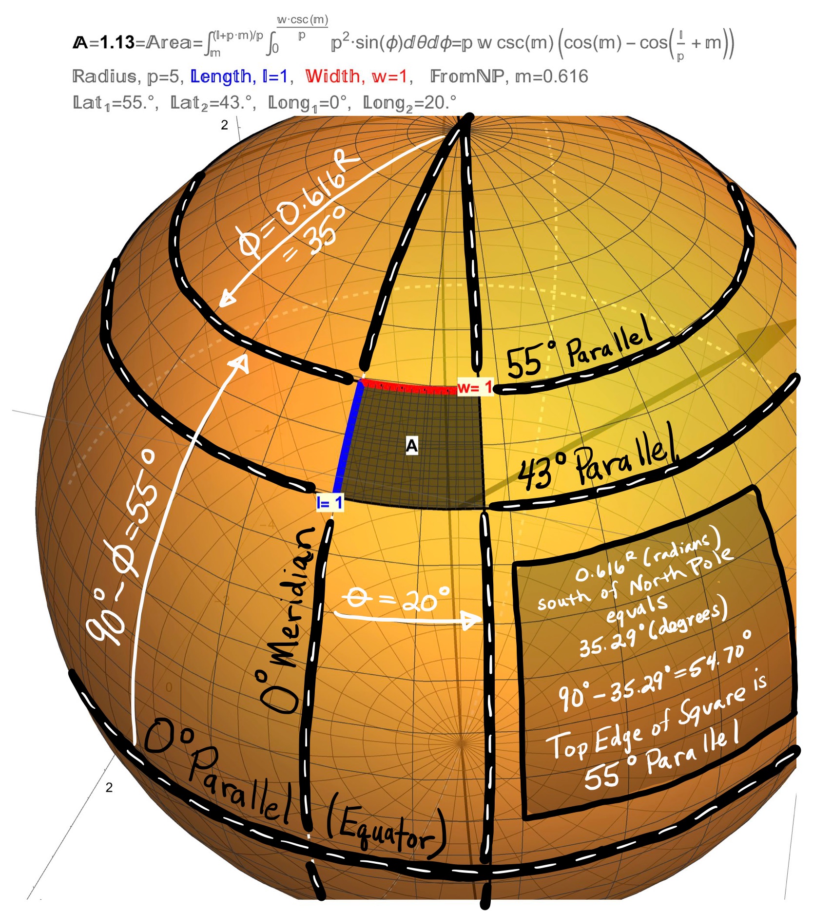
Figure 3: Special Curves and Regions On a Sphere: Describe the sphere parametrically as \(r(\theta,\phi)=(\rho\sin(\phi)\cos(\theta),\rho\sin(\phi)\sin(\theta),\rho\cos(\phi))\) with \(\theta\) the Longitude angle (measured from the Prime Meridian) and \(\phi\) the Latitude angle (measured from the North Pole). The Meridians are the circles of constant Longitude \(\theta=k\) given by \(r(\phi)=(\rho\sin(\phi)\cos(k),\rho\sin(\phi)\sin(k),\rho\cos(\phi))\). The Parallels are the circles of constant Latitude \(\phi=c\) given by \(r(\theta)=(\rho\sin(c)\cos(\theta),\rho\sin(c)\sin(\theta),\rho\cos(c)).\) A Special Parallel is the Equator (\(\phi=c=\pi/2\)) given by \(r(\theta)=(\rho\cos(\theta),\rho\sin(\theta),0)\). A Special Meridian is the Prime Meridian (\(\theta=k=0\)) given by \(r(\phi)=(\rho\sin(\phi),0,\rho\cos(\phi))\).
If the Earth was a Sphere of Radius \(\rho=5\) then…
…The images in Figures 1, 2, 3 would looks like those seen in Figures 4 and 5.
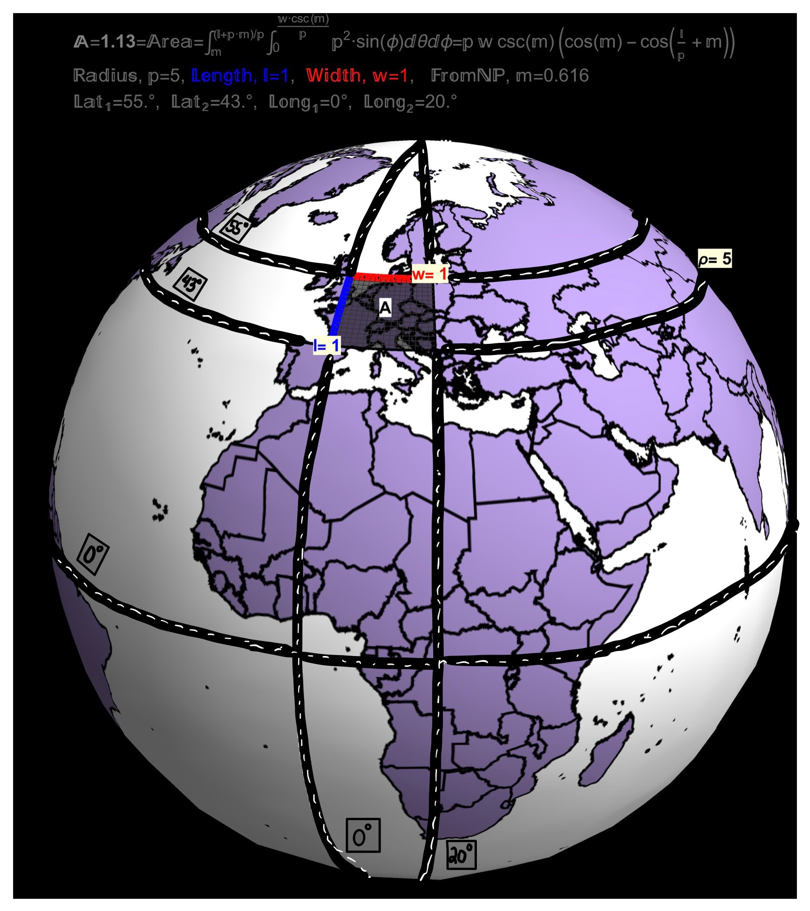
Figure 4: If the Earth was a Sphere of Radius \(\rho=5 (cm)\)… The \(\theta=0\) Line of Longitude is called the Prime Meridian and passes through England (particularly, Greenwich). The \(\phi=\pi/2\) Line of Latitude is called the Equator.
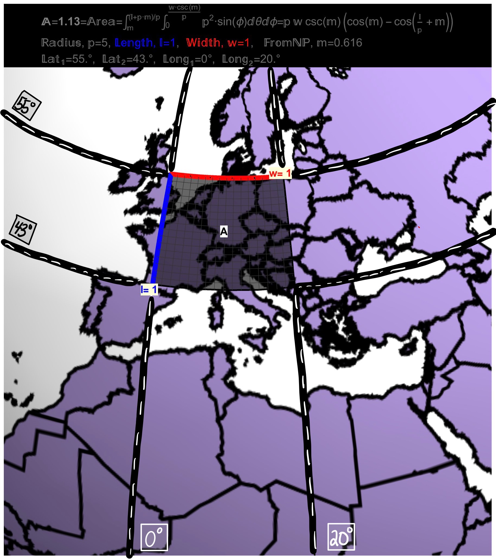
Figure 5: If the Earth was a Sphere of Radius \(\rho=5 (cm)\)…A square of dimension \(1 \,(cm) \;\times \;1\, (cm)\) between the Parallels \(55^{\circ}\) and \(43^{\circ}\) is shown which covers \(20^\circ\) of Longitude and has an area of 1.13 (\(cm^{2}\)).
A Reminder About Circles, Radians, and Degrees
In the animated graphic novel On Maps and Maths and Making Friends: A Curvature Story, the characters Pete and Brenna need to refresh their own memories about the concept of a radian and it’s relationship to a circle. Figures 6 and 7 are snapshots of their notes (from the book).
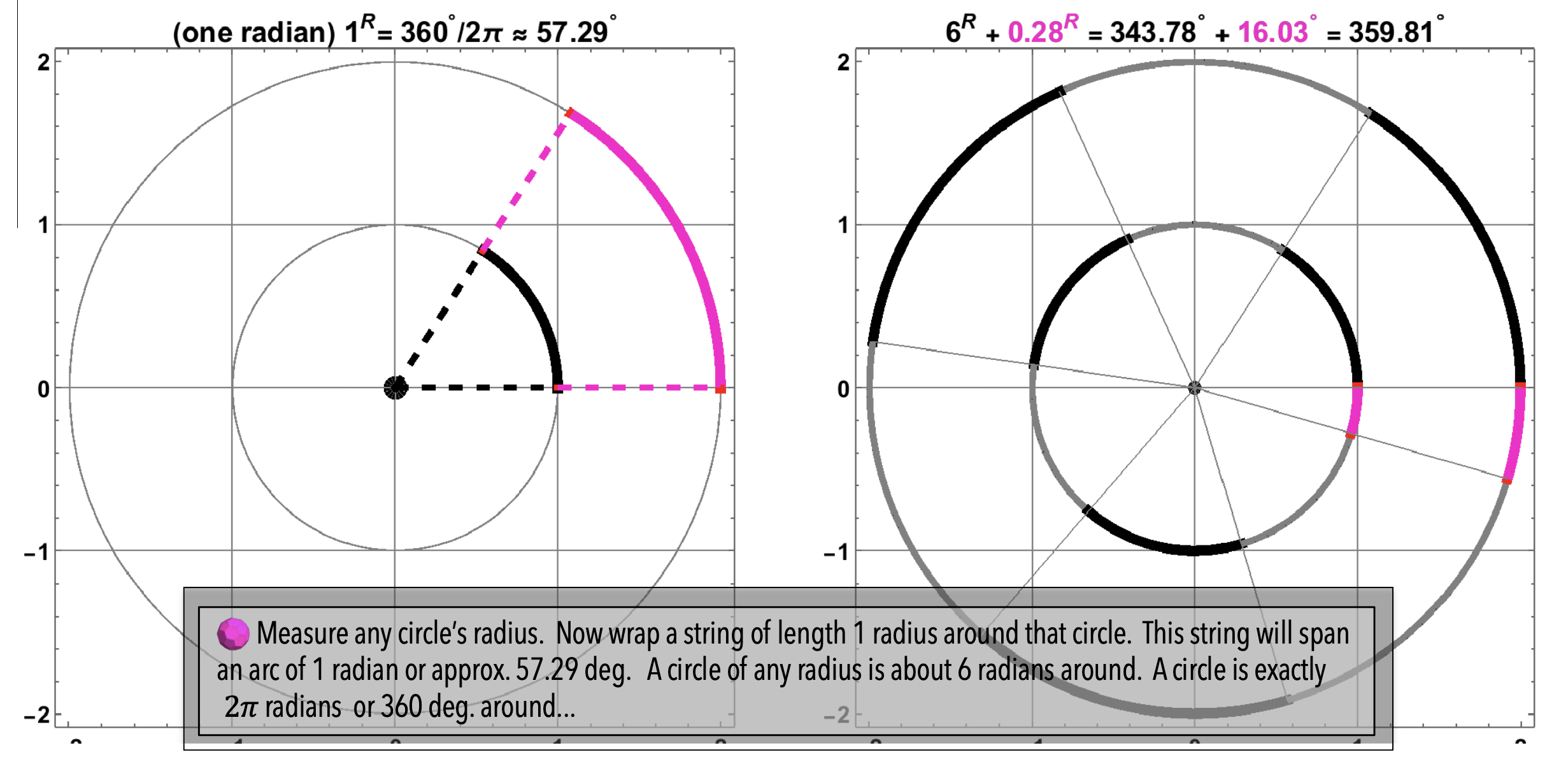
Figure 6: On Radians: One radian (\(1^{R}\)) is about fifty-seven degrees (\(57^{\circ}\)). There are \(2\pi\) radians (or about six and one-forth radians) in one full circuit (\(360^{\circ}\)) of a circle.
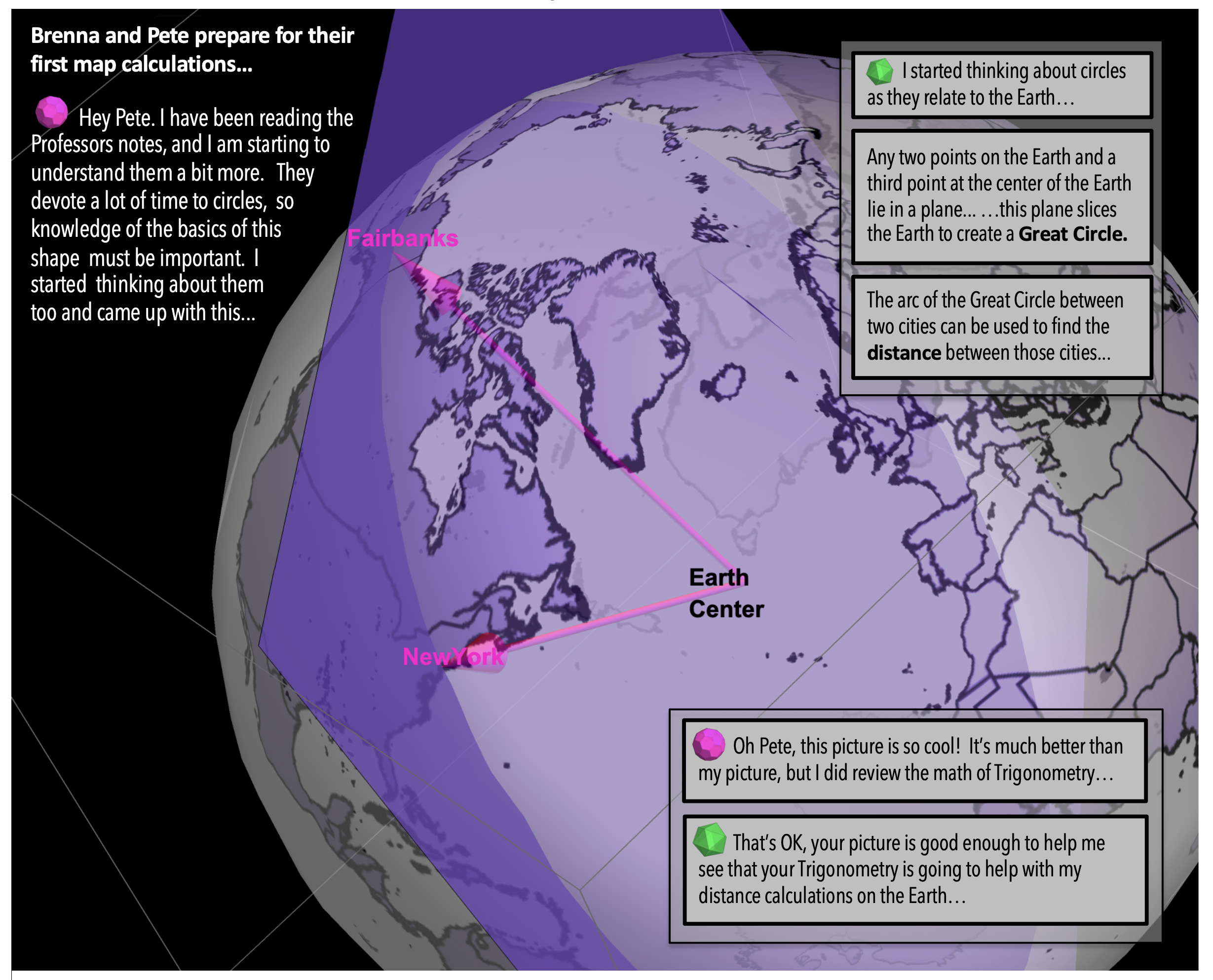
Figure 7: On Radians: When a plane derived from two points on a sphere and the center of the sphere intersects the sphere itself, the resulting curve is a Great Circle.
The Relationship Between Length and Width Distances and Latitude and Longitude on a Sphere
The key to defining a square on a sphere as the region between two equally spaced Latitudes and two Longitudes is being able to correctly determine distances on a sphere. To illustrate how distance is related to latitude and longitude consider the situation summarized by
- There are two running-roommates (one red, one blue) who live in a house on a sphere of radius of 5 (miles) at latitude \(\phi=0.616^{R}\) and longitude \(\theta=0^{R}\).
- Each roommate will run 1 (mile) according to the pedometers they have on their smart watches, but they will run in different directions. The blue roommate will leave the start (home) and run along a line of longitude for the 1 (mile). The red roommate will run for 1 (mile) along a line of latitude.
- A Question is “After running 1 (mile), what are the finishing locations in latitude (\(\phi\)) and longitude (\(\theta\)) of each runner?”
This situation is illustrated in Figures 8 and 9.
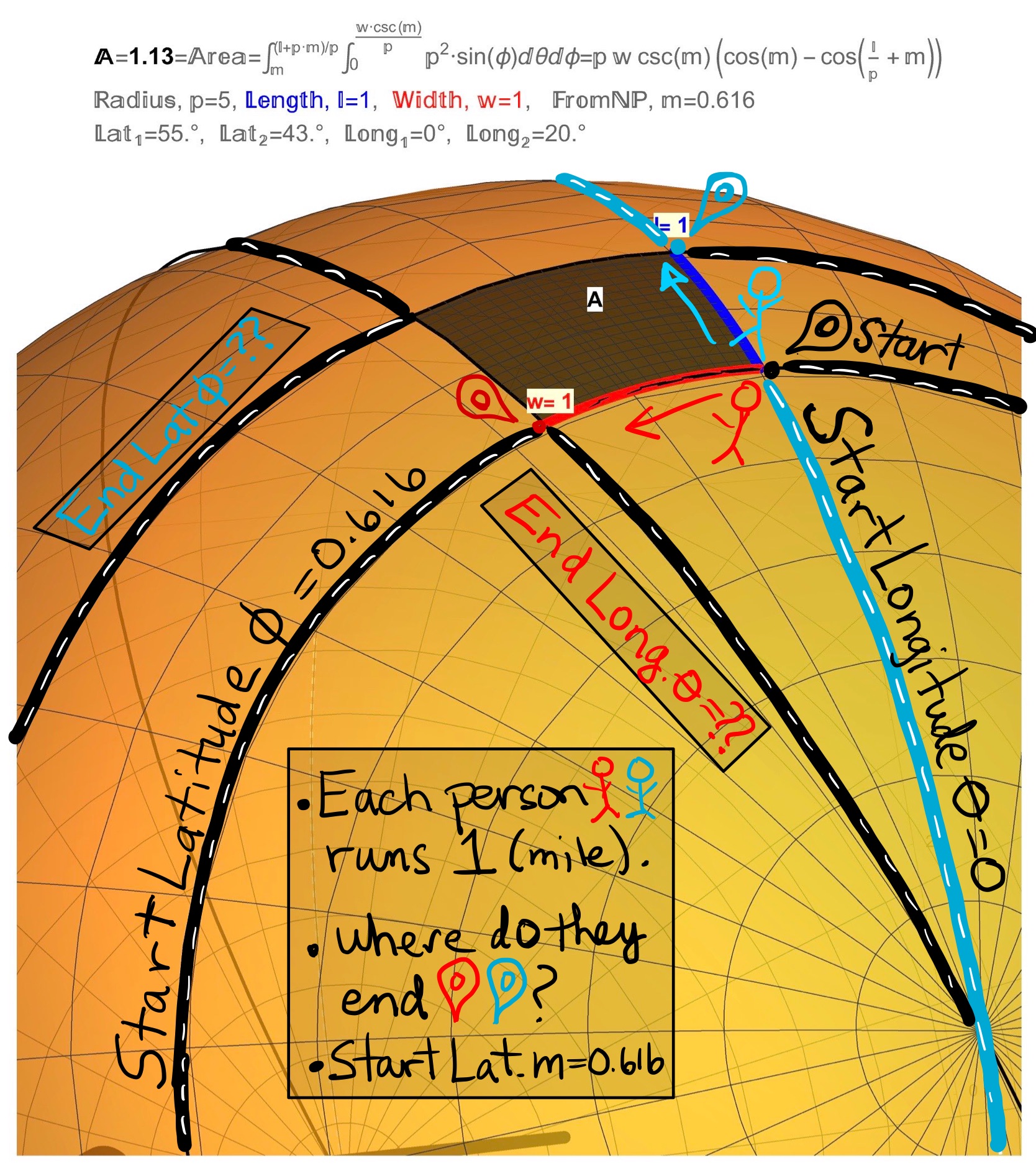
Figure 8: Question: If two runners (blue and red) both start at the location \((\theta,\phi)=(0^{R},0.616^{R})\) on a sphere of radius 5 (miles) and run for 1 (mile) (but in opposite directions; along a longitude and latitude, respectively), then what is the finishing location \((\theta,\phi)\) of each runner? The question applies equally to airplanes and flight paths.
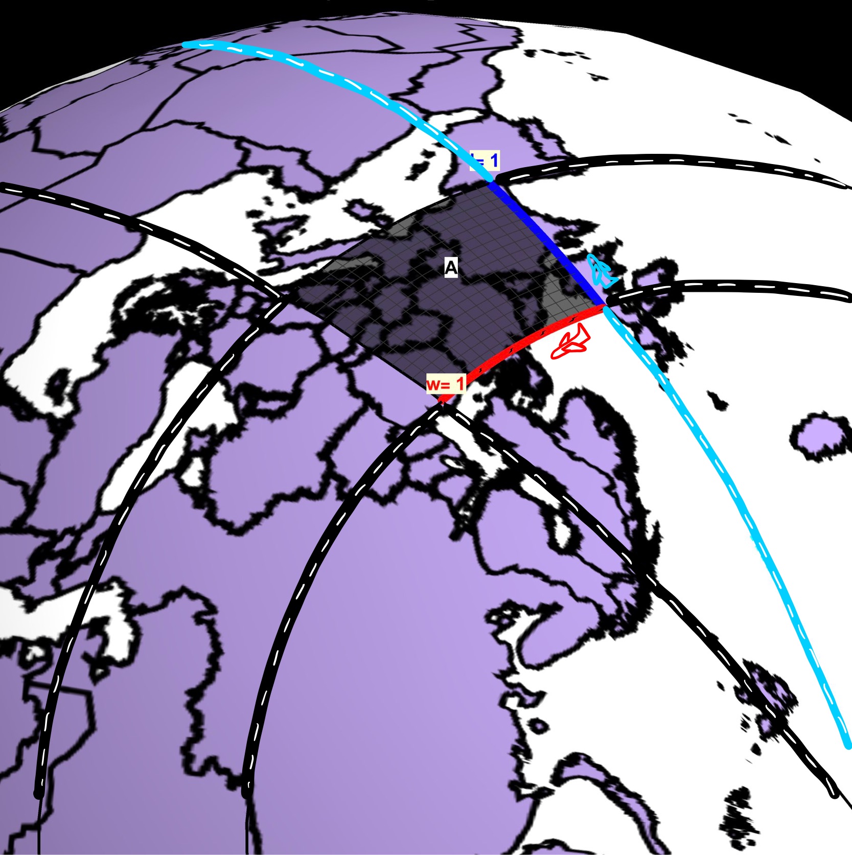
Figure 9: The same question in Figure 8 applies equally to airplanes and flight paths.
The Answer to the Question posed in Figure 8 begins to take shape when we realize that
Because the blue runner is always on the \(\theta=0\) longitude, their finish location will be \((\theta,\phi)=(0,\phi=?)\) for some as yet to be determined value of \(\phi\).
Similarly, the red runner is always on the \(\phi=0.616\) latitude, so they will have to finish at \((\theta,\phi)=(\theta=?,0.616)\) for some value we need to find \(\theta\).
Because each runner is on a sphere, the paths they are running along must also curve with the sphere. Mathematically speaking, the curve for the blue runner is \[\begin{align} r(\phi)&=r(\rho=5,\theta=0,\phi)\\ &=(5\sin(\phi),0,5\cos(\phi)), \end{align}\] while for the red runner the curve is \[\begin{align} r(\theta)&=r(\rho=5,\theta,\phi=0.616)\\ &=(2.88\cos(\theta),2.88\sin(\theta),4.08). \end{align}\] The length (l) and width (w) distances run along these curves are given by (arc-length) integrals \[\begin{align} l(\phi)&= \int_{\phi=0.616}^{\phi}\sqrt{\frac{dr}{d\phi}\cdot \frac{dr}{d\phi}}\; d\phi=5\phi-3.08 \\ w(\theta)&= \int_{\theta=0}^{\theta}\sqrt{\frac{dr}{d\theta}\cdot \frac{dr}{d\theta}}\; d\theta=2.88\theta. \end{align}\] Since each runner is to run a distance of 1 (mile) then solving the equations \[\begin{align} l(\phi) &=1=5\phi-2.08 \\ &\implies \phi=0.816=3.08/5, \\ w(\theta) &=1=2.88\theta \\ &\implies \theta=0.346=1/2.88. \end{align}\]
That is, if the blue runner starts at \((\theta,\phi)=(0,0.616)\) and finishes at \((\theta,\phi)=(0,0.816)\), then they will have run \(l=1\) (mile). In other words, at a starting latitude of \(\phi=0.616\) a distance of \(l=1\) mile corresponds to a change in latitude \(\Delta \phi=0.81-0.61=0.2^{R}\).
Similarly, if the red runner starts at \((\theta,\phi)=(0,0.616)\) and finishes at \((\theta,\phi)=(0.346,0.616)\), then they will also have run \(w=1\) (mile). However, in contrast, at a starting latitude of \(\phi=0.616\) a distance of \(w=1\) mile corresponds to a change in longitude \(\Delta \theta =0.346-0=0.346^{R}\) (a greater change than \(\Delta \phi=0.2\)!). In other words, at a starting latitude of \(\phi=0.616\), a \(w=1\) (mile) covers more longitudial distance than a \(l=1\) (mile) covers latitudinal distance.
The area of the square created by both runners on a sphere of radius \(\rho=5\) at starting latitude \(m=0.616\) is given by the (surface area) integral \[\begin{align} A&=\int_{\phi=0.616}^{\phi=0.816} \int_{\theta=0}^{\theta=0.346} 25\sin(\phi)\;d\theta \; d\phi\\ &=1.13 \;(\mbox{miles}^{2}). \end{align}\]
These computations are illustrated and summarized in Figure 10.
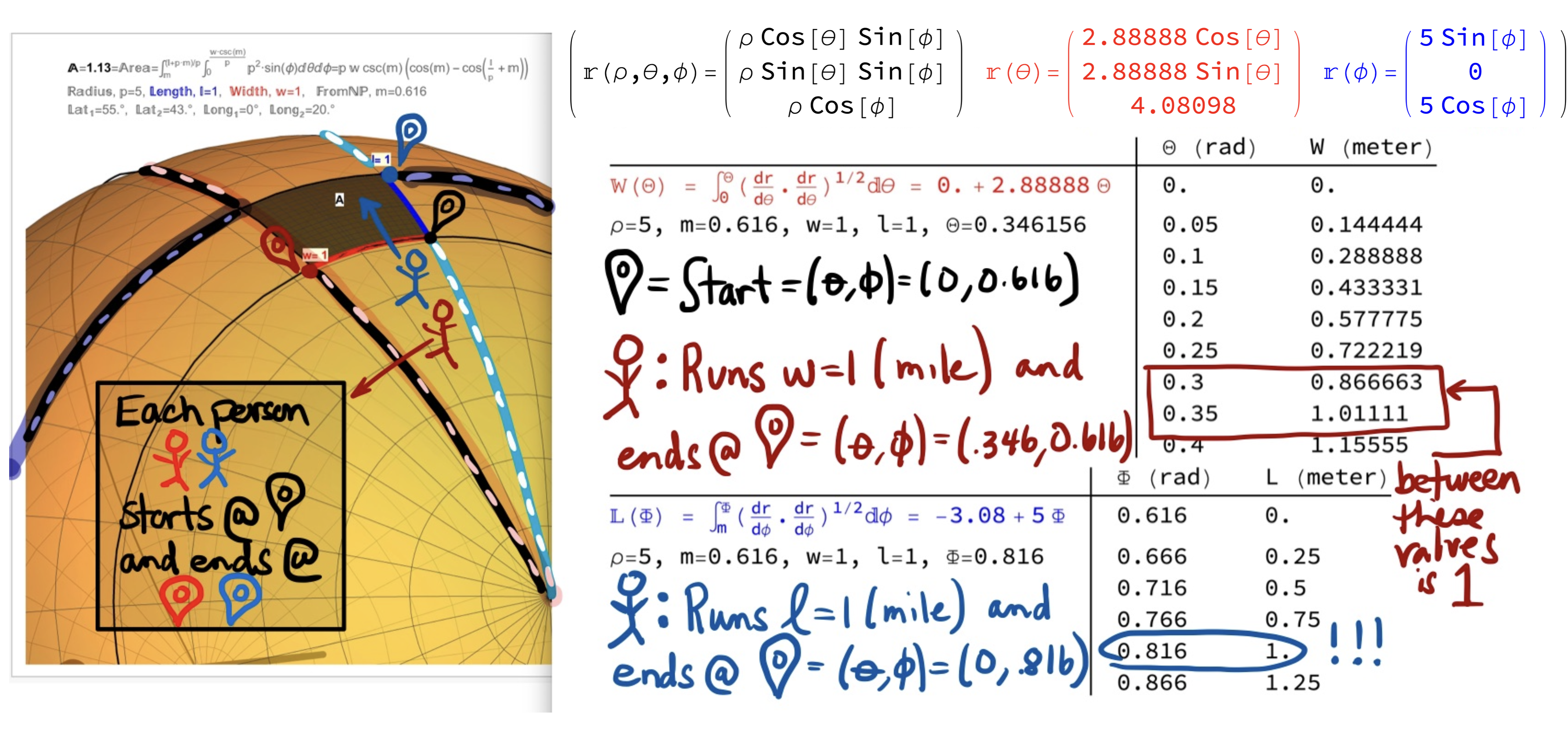
Figure 10: Limits of (Surface Area) Integral Justification at \(\phi=m=0.616^{R}\): The table of values for the red runner shows that as they cross the lines of longitude \(\phi=0.1\) and \(\phi=0.3\) the distances run are \(w=.289\) and \(w=0.866\), respectively. To run a distance of exactly \(w=1\) requires the red runner to travel to a line of longitude of approximatley \(\phi >0.3\). The table of values for the blue runner shows them crossing the lines of latitude \(\phi=0.716\) and \(\phi=0.816\) for a distance of \(l=0.5\) and \(l=1\), respectively.
Limits of Area Justification: At Any Starting Latitude \(\phi=\mathbb{M}\)
In general, the question posed in Figure 8 can be extended to a sphere of any radius \(\rho\), any starting latitude \(\mathbb{M}\), and for a rectangle of any length \(\mathbb{L}\) and width \(\mathbb{W}\). In this general case the arc-length integrals for the edges of sphere rectangle are
\[\begin{align} l(\Phi)&= \int_{\phi=\mathbb{M}}^{\Phi}\sqrt{\frac{dr}{d\phi}\cdot \frac{dr}{d\phi}}\; d\phi=\mathbb{L}, \\ w(\Theta)&= \int_{\theta=0}^{\Theta}\sqrt{\frac{dr}{d\theta}\cdot \frac{dr}{d\theta}}\; d\theta=\mathbb{W}. \end{align}\]
These equations can be solved for \(\Theta\) and \(\Phi\) in Mathematica as seen in Figure 11 to obtain
\[\begin{align} \Theta =\frac{\mathbb{W}\csc(\mathbb{M})}{\rho} \;\; \mbox{and} \;\; \Phi=\frac{\mathbb{L} + \mathbb{M}\rho}{\rho}. \end{align}\]
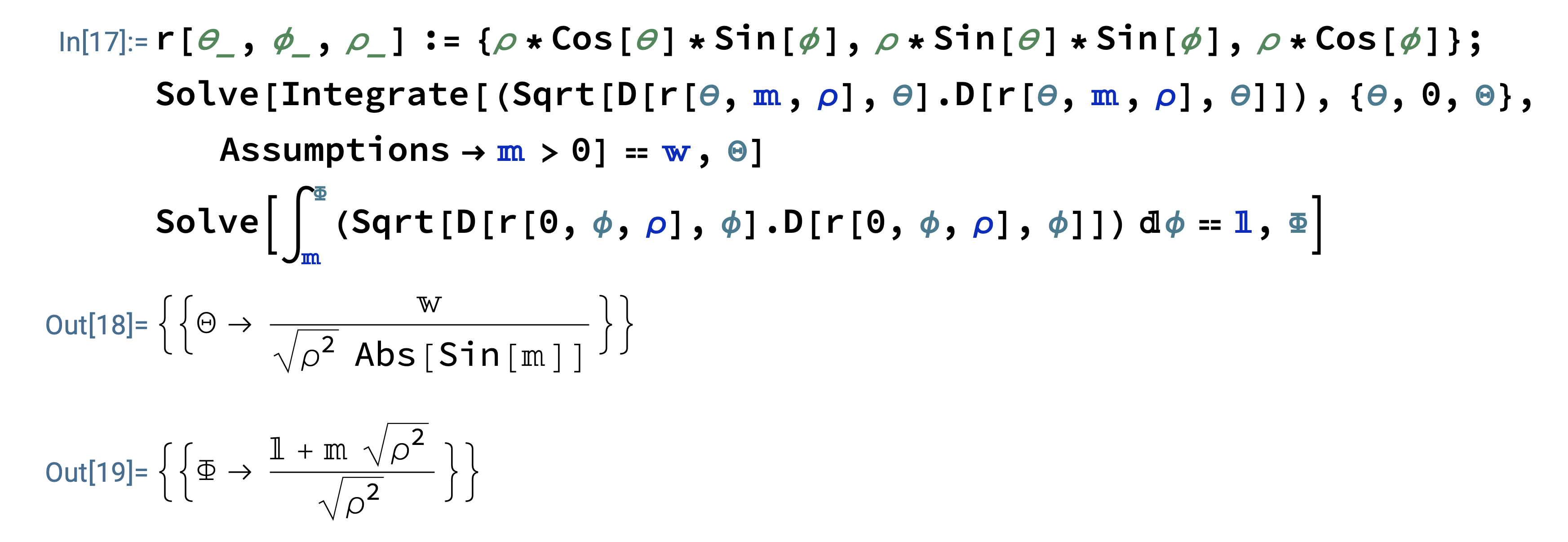
Figure 11: Example Mathematica Code Which Solves for the Latitude and Longitude Angles \(\Phi\) and \(\Theta\).
With these angles it is now possible to setup and evaluate the (surface area) integral for the area \(\mathbb{A}\) of a \(\mathbb{L} \times \mathbb{W}\) rectangle on a sphere of any radius \(\rho\) and any starting latitude \(\mathbb{M}\),
\[\begin{align} \mathbb{A}&= \int_{\phi=\mathbb{M}}^{\phi=\frac{\mathbb{L}+\mathbb{M}\rho}{\rho}}\int_{\theta=0}^{\theta=\frac{\mathbb{W}\csc(\mathbb{M})}{\rho}} \rho^{2}\sin(\phi)\; d\theta\; d\phi\\ &=\rho \mathbb{W} \csc(\mathbb{M})\left(\cos(\mathbb{M})-\cos\left(\frac{\mathbb{L}}{\rho}+\mathbb{M}\right) \right). \end{align}\]
Two Results for the Area of a \(1 \times 1\) Square on a Sphere
Bringing all of the skills and results from above together we get the animations shown in Figures 12 and 14.
Figure 12: Result 1: The area of a \(1 \times 1\) square on a sphere changes with latitude.
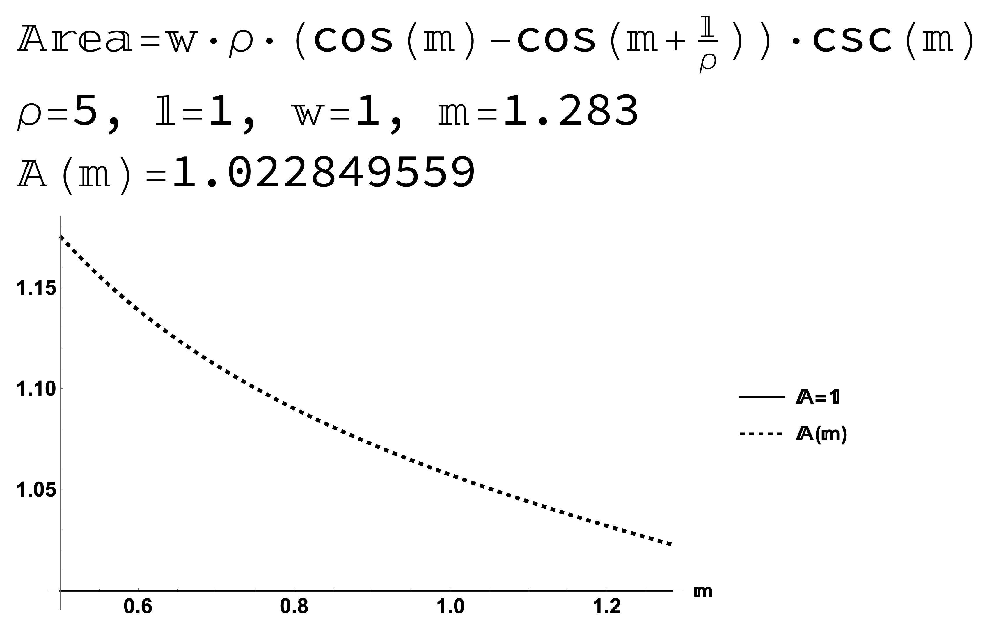
Figure 13: Result 1: The area of a \(1 \times 1\) square on a sphere changes with latitude.
Figure 14: Result 2: The area of a \(1 \times 1\) square on a sphere approaches \(A=1\) as the radius of the sphere \(\rho\) increases.
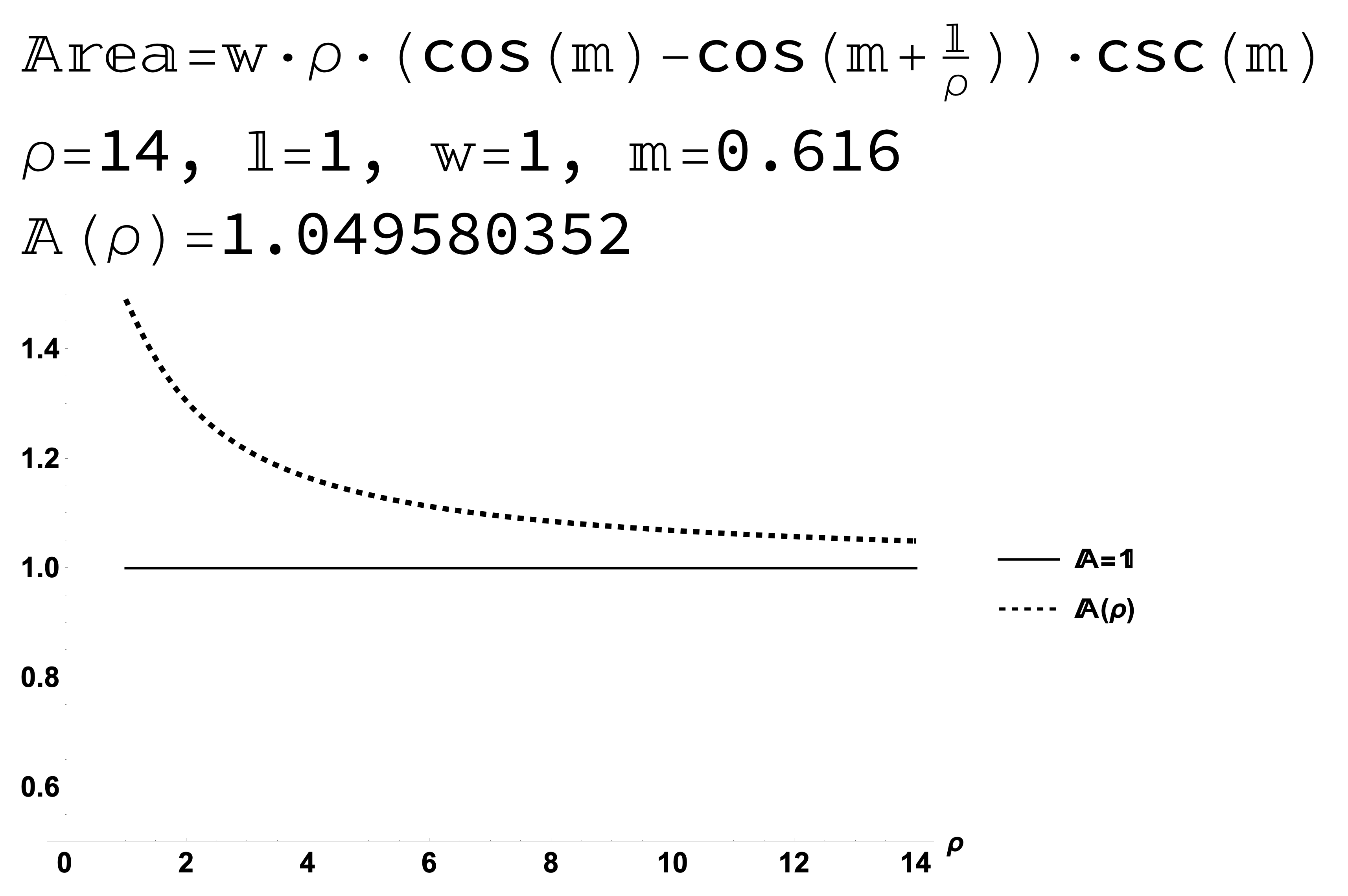
Figure 15: Result 2: The area of a \(1 \times 1\) square on a sphere approaches \(A=1\) as the radius of the sphere \(\rho\) increases.
If the Earth was a Sphere of Radius \(\rho=6378 (km)\) then…
…This would be a pretty accurate representation as NASA shows this number as the equatorial radius of the Earth. Further, a \(1 (km) \times 1 (km)\) square at a starting latitude \(\phi=0.83^{R}\) (from North Pole) or \(42^{\circ}N\) (from Equator) on the Earth according to Google Earth will look like the region of Figure 16 and have an area shown in Figure 17.

Figure 16: Zoom In: Assuming the Earth is a sphere of radius \(\rho=6378km\), one has to zoom quite a lot in Google Earth to make out a \(1km \times 1km\) square on the \(42^{\circ}N\) parallel. This region of Iowa was selected for viewing because of the flat farmland of the area (more on this shortly).
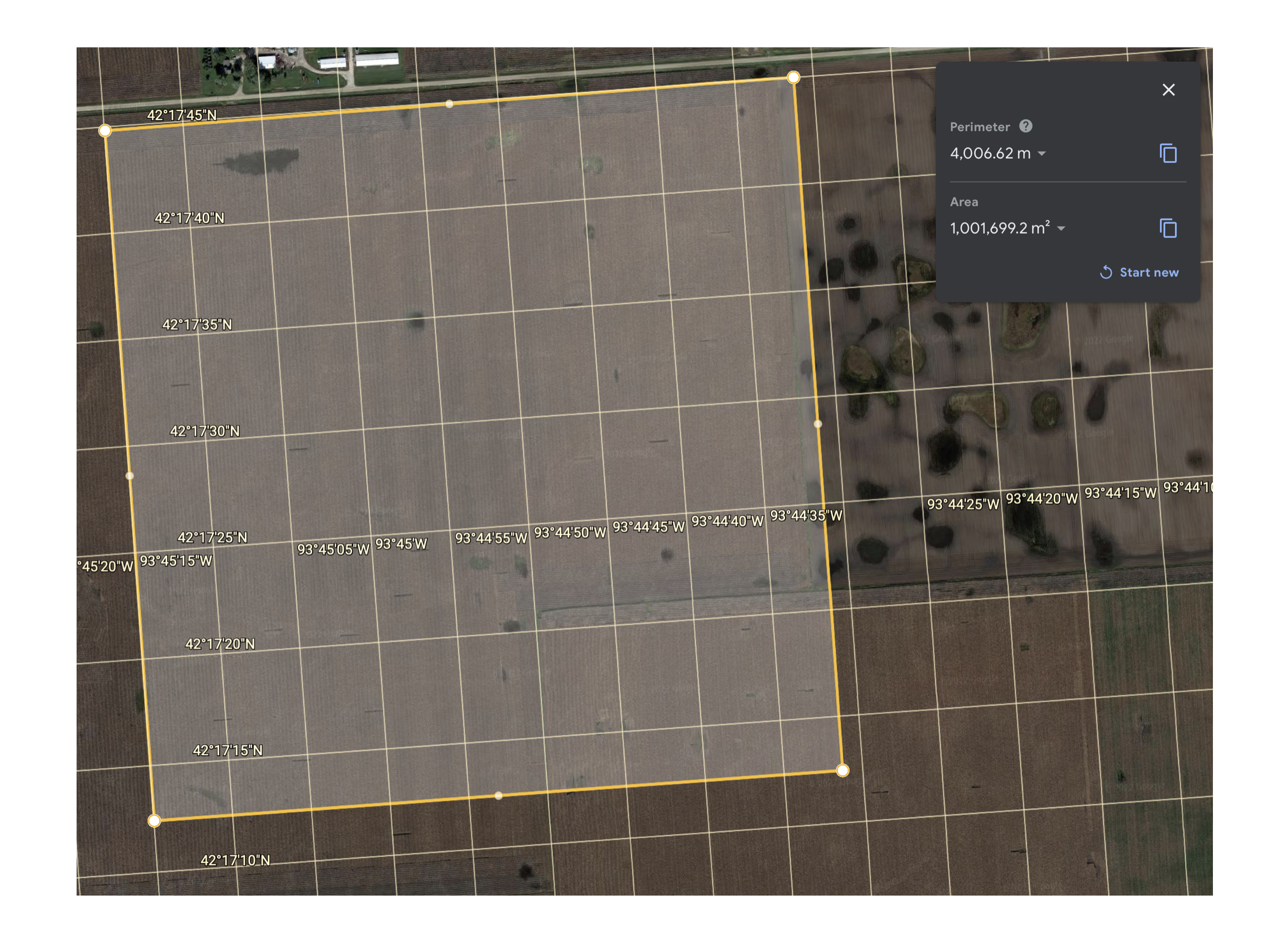
Figure 17: Measurements from Google Earth: Using the available (but likely imprecise measurement tools of Google Earth) the area of this \(1km \times 1km\) square at latitude \(\phi=0.83^{R}\) is approximately \(1km^{2}+1,700m^{2}\) which is clearly greater than \(1km^{2}\). The extra area is due to the curvature of the Earth.
Using the area function \(\mathbb{A}\) as seen in Figure 18, computes the area of this region to be approximately \(A=1km^{2}+0.000072km^{2}=1km^{2}+72m^{2}\), which we note is greater than \(1km^{2}\) but not really by that much.
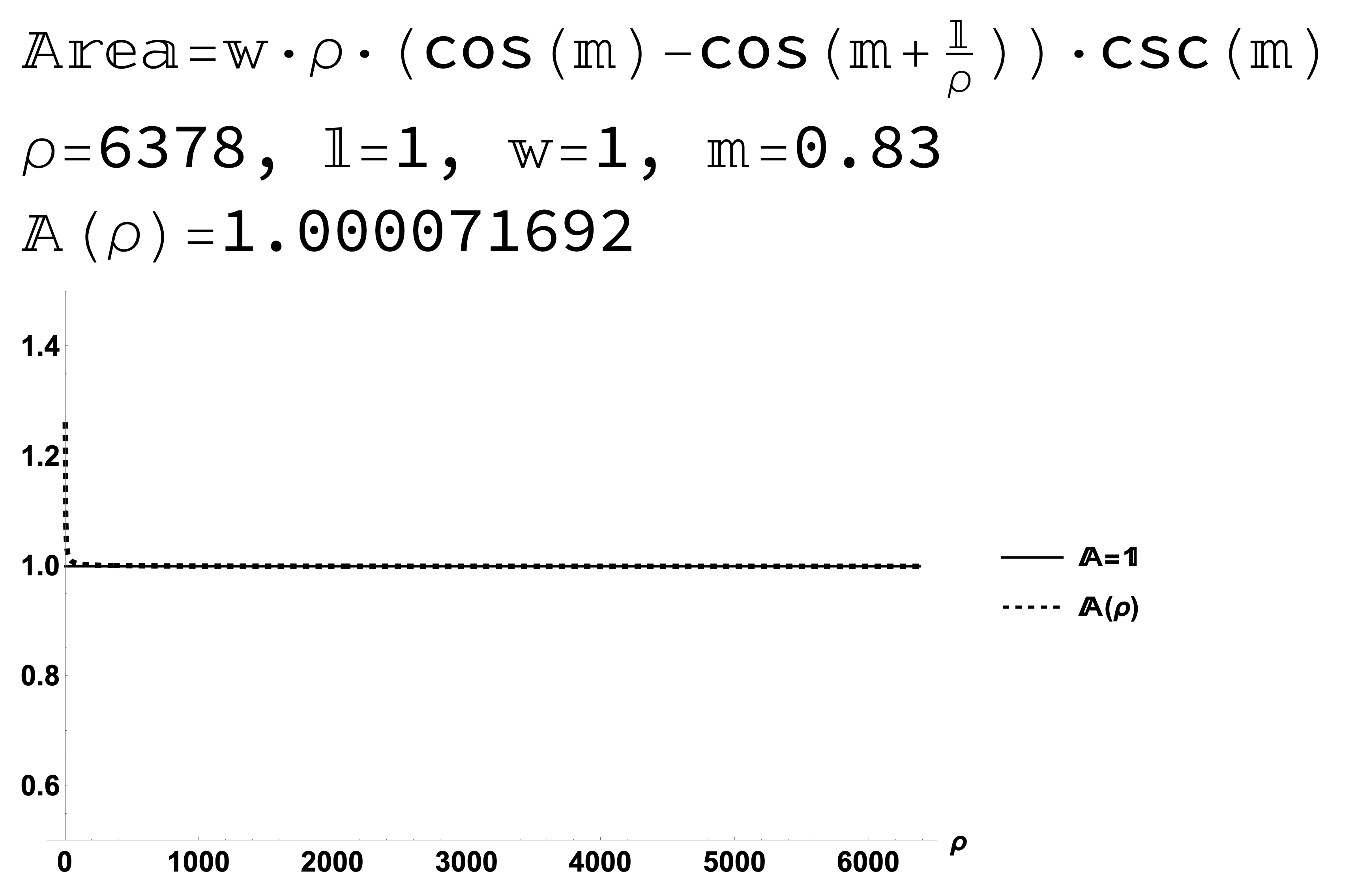
Figure 18: The area of a \(1km \times 1km\) square on the parallel \(42^{\circ}N\) of the Earth (\(\rho=6378km\)) is approximately \(A=1km^{2}+72m^{2}\). This extra area is as close as I can get to quantifying the effects the Earth’s curvature has on areas (assuming of course that not only are my calculations correct, but also without assuming the Earth is an ellipsoid which would require us to adjust all of the above computations).
And Now…The Cost of Curvature
To put these area numbers into context, assume that you are a farmer in Iowa at \(42^{\circ}N\) who needs to fertilize one of your \(1km \times 1km\) fields.
If you purchased exactly \(1km^{2}\) (essentially \(247 acres\)) of fertilizer then (at \(\$50/acre\)) while you would have spent a total of \(\$12,350\) you still would have come up short by \(72m^{2}\) (essentially \(0.02\) acres). The cost estimate of fertilizer came from my brother-in-law who is farmer in Northwest Pennsylvania.
To finish the field you would need an additional \(\$1=\$50/acre\cdot 0.02acre\) of fertilizer for a total cost of \(\$12,351\). In other words, the cost of curvature to fertilize the field is \(\$1\)!
That is, the cost of curvature is \(0.008\%\) of the total costs to fertilize the field. While this is indeed a small percentage it does accurately reflect the costs of curvature. However, at the large radii of the Earth, the curvature effects are almost negligible from a cost perspective in this particular application…of fertilizer (pun intended).
In a Future Post…
…We will delve further into great circles (or geodesics of the sphere), as we attempt to find a better way to connect the quantification of the curvature \(\kappa\) of a sphere of radius \(\rho\) given by the formula \[\begin{align} \kappa=\frac{1}{\rho^{2}} \end{align}\] with the area of, not a square as shown in this post, but rather a special triangle called a geodesic triangle on the sphere.