Geodesic Triangles on Sphere

In this post we illustrate the interest that Differential Geometers (those folks who like to mix Calculus with Geometry) have with the concepts of curvature and geodesics. We illustrate curvature as that deviant quality inherent to a sphere which deforms the standard Euclidean result requiring that angles of a triangle add to \(180^{\circ}\). We also see that in defining the Differential Geometric equivalent of straight lines (geodesics), the mathematical and computational complexities increase drastically. This is the first post which illustrates the Maple package I have written (called tensorAddOns) whose purpose is to handle the difficult computations involving many of the higher dimensional objects in Differential Geometry.

Last Updated: Sunday, October 02, 2022 - 15:29:34.

What Has Gone On Before…

In the post Cost of Curvature the area \(\mathbb{A}\) of a \(\mathbb{L} \times \mathbb{W}\) rectangle on a sphere of any radius \(\rho\) and any starting latitude \(\mathbb{M}\) was shown to be

\[\begin{align} \mathbb{A}&= \int_{\phi=\mathbb{M}}^{\phi=\frac{\mathbb{L}+\mathbb{M}\rho}{\rho}}\int_{\theta=0}^{\theta=\frac{\mathbb{W}\csc(\mathbb{M})}{\rho}} \rho^{2}\sin(\phi)\; d\theta\; d\phi\\ &=\rho \mathbb{W} \csc(\mathbb{M})\left(\cos(\mathbb{M})-\cos\left(\frac{\mathbb{L}}{\rho}+\mathbb{M}\right) \right). \end{align}\]

Specifically the area of a \(\mathbb{L}=1\) by \(\mathbb{W}=1\) square on a sphere at starting latitude \(\mathbb{M}=0.616\) is \[\begin{align} \mathbb{A}&=\rho \csc(\mathbb{M})\left(\cos(\mathbb{M})-\cos\left(\frac{1}{\rho}+\mathbb{M}\right) \right)\\ &\approx 1.731\rho\left(0.816-\cos\left(\frac{1}{\rho}+0.616 \right) \right). \end{align}\]

As seen in Figures 1 and 2, a result of this formula is that the area of a \(1 \times 1\) square on a sphere approaches \(A=1\) as the radius of the sphere \(\rho\) increases.

Figure 1: Result: The area of a \(1 \times 1\) square on a sphere approaches \(A=1\) as the radius of the sphere \(\rho\) increases.

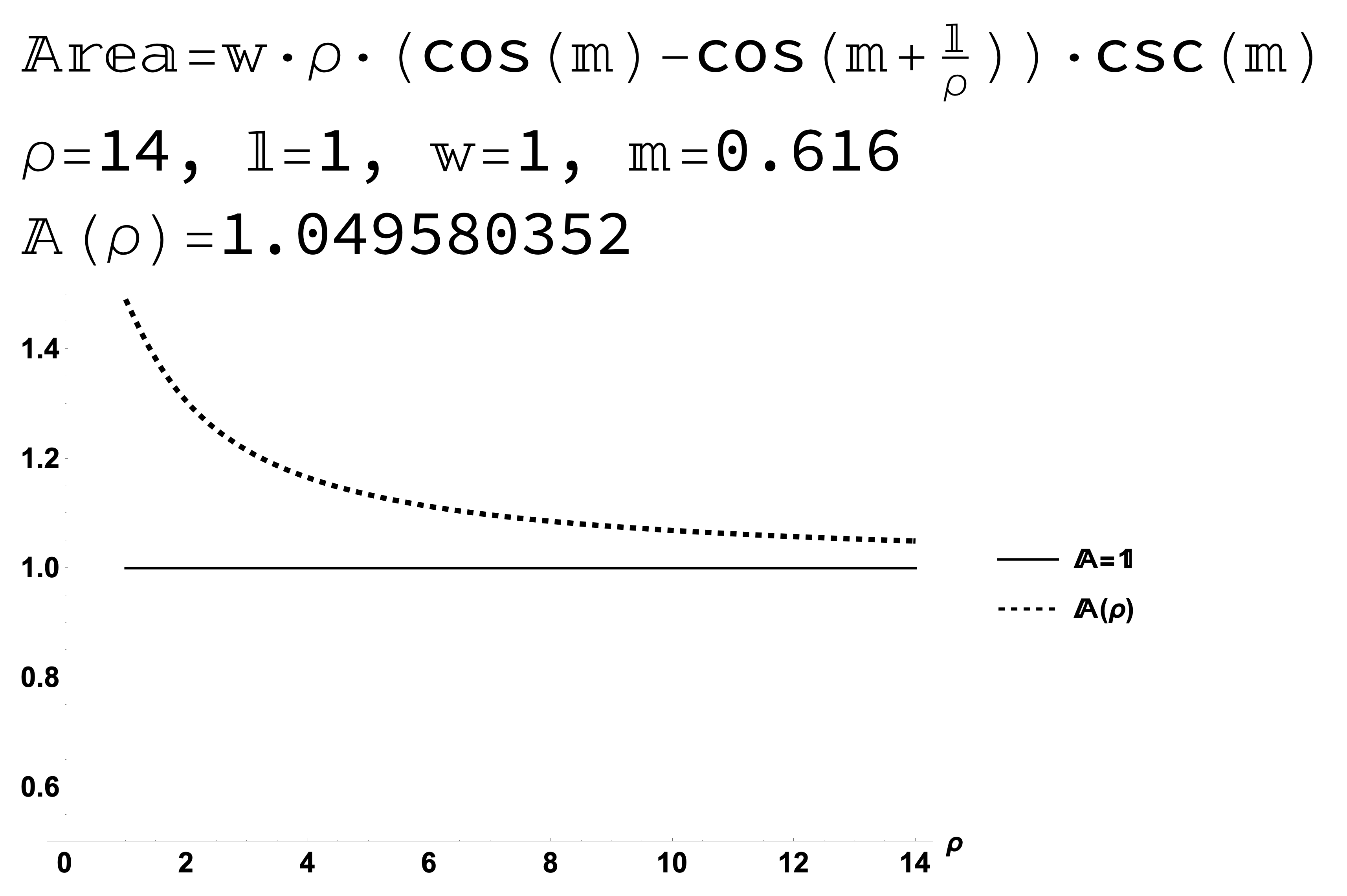
Figure 2: Result: The area of a \(1 \times 1\) square on a sphere approaches \(A=1\) as the radius of the sphere \(\rho\) increases.

Note that what we do not see in this area–of–rectangles–on–a–sphere result is an ideal formula that simplifies to something like \[\begin{align} \mathbb{A}&=\mathbb{L}\mathbb{W}+\mathbb{N}(\rho), \end{align}\] where \(\mathbb{N}(\rho)\) is some \(\mathbb{N}\)umber that changes with the radius \(\rho\) and diminishes to \(0\) as \(\rho\) gets larger. A formula of this type would be ideal for the following reasons:

• The known area of a \(\mathbb{L} \times \mathbb{W}\) rectangle drawn on a flat sheet of paper (a Euclidean rectangle) is \(\mathbb{A}=\mathbb{L}\mathbb{W}\)

• If the area of a \(\mathbb{L} \times \mathbb{W}\) rectangle drawn on a sphere of radius \(\rho\) were in fact \(\mathbb{A}=\mathbb{L}\mathbb{W}+\mathbb{N}(\rho)\) such that \(\mathbb{N}(\rho)\rightarrow 0\) as \(\rho\rightarrow \infty\) then this would conveniently show that the Euclidean Limit of the rectangle area on the sphere is the Euclidean rectangle area.

Unfortunately, this ideal result is not reality. Instead we have the complicated formula for rectangular area on a sphere \[\begin{align} \mathbb{A}&=\rho \mathbb{W} \csc(\mathbb{M})\left(\cos(\mathbb{M})-\cos\left(\frac{\mathbb{L}}{\rho}+\mathbb{M}\right) \right) \\ &\neq \mathbb{L}\mathbb{W}+\mathbb{N}(\rho). \end{align}\]

In this post, we illustrate that by switching to areas of (geodesic) triangles on a sphere then there is an ideal formula \[\begin{align} \pi+\mathbb{N}(\rho)=\pi+\frac{\mathbb{A}}{\rho^{2}}, \end{align}\] where \(\mathbb{A}\) is the area of a (geodesic) triangle from which a natural Euclidean Limit will follow. To understand this formula requires then the introduction of new idea called a geodesic.

Recall the Definitions…Meridians (Lines of Longitude) and Parallels (Line of Latitude)

Mathematically, we can describe a sphere of radius \(\rho\) parametrically as \[\begin{align} r(\theta,\phi)&=(f(\phi)\cos(\theta),f(\phi)\sin(\theta),h(\phi)), \end{align}\] where \[\begin{align} f(\phi)=\rho\sin(\phi)\;\; \mbox{and}\;\; h(\phi)=\rho\cos(\phi). \end{align}\] In this parameterization, \(\theta^{R}\) is the angle (in radians) from the Prime Meridian to a Line of Longitude while the \(\phi^{R}\) is the angle (in radians) from the North Pole to a Line of Latitude. The value \(\psi^{\circ}=90^{\circ}-\phi^{\circ}\) is therefore the angle in degrees from the Equator to a Line of Latitude. The value \(\psi^{\circ}=90^{\circ}-\phi^{\circ}\) can also be called the \(\psi^{\circ}\)th Parallel.

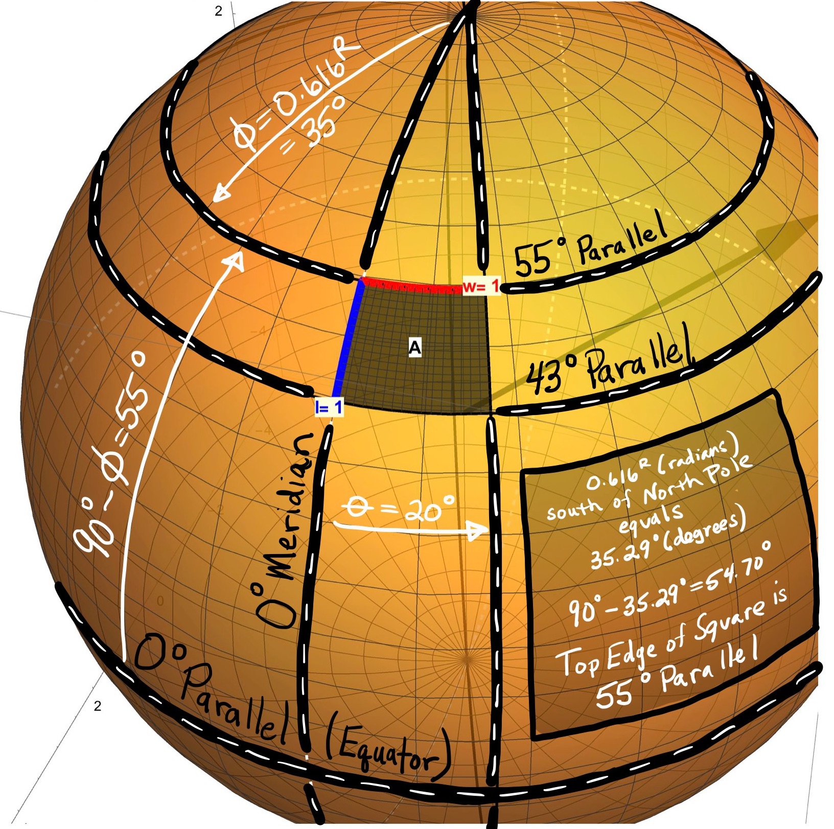
Figure 3: Special Curves On a Sphere: Describe the sphere parametrically as \(r(\theta,\phi)=(\rho\sin(\phi)\cos(\theta),\rho\sin(\phi)\sin(\theta),\rho\cos(\phi))\) with \(\theta\) the Longitude angle (measured from the Prime Meridian) and \(\phi\) the Latitude angle (measured from the North Pole). The Meridians are the circles of constant Longitude \(\theta=k\) given by \(r(\phi)=(\rho\sin(\phi)\cos(k),\rho\sin(\phi)\sin(k),\rho\cos(\phi))\). The Parallels are the circles of constant Latitude \(\phi=c\) given by \(r(\theta)=(\rho\sin(c)\cos(\theta),\rho\sin(c)\sin(\theta),\rho\cos(c)).\) A Special Parallel is the Equator (\(\phi=c=\pi/2\)) given by \(r(\theta)=(\rho\cos(\theta),\rho\sin(\theta),0)\). A Special Meridian is the Prime Meridian (\(\theta=k=0\)) given by \(r(\phi)=(\rho\sin(\phi),0,\rho\cos(\phi))\).

The Equator and all Lines of Longitude and the Great Circles are Geodesics on a Sphere

Without yet getting into technical details, let’s state that the geodesics on a sphere, seen in Figure 4, are

• The Equator (a special Parallel)
• All Lines of Longitude (including the Prime Meridian)
• And any Great Circle between two points \(P\) and \(Q\) on the sphere. A great circle can be described as the circle of intersection of the sphere and a special plane obtained from any two distinct points on the sphere \(P\) and \(Q\) and the center of the sphere \(\cal{O}\).

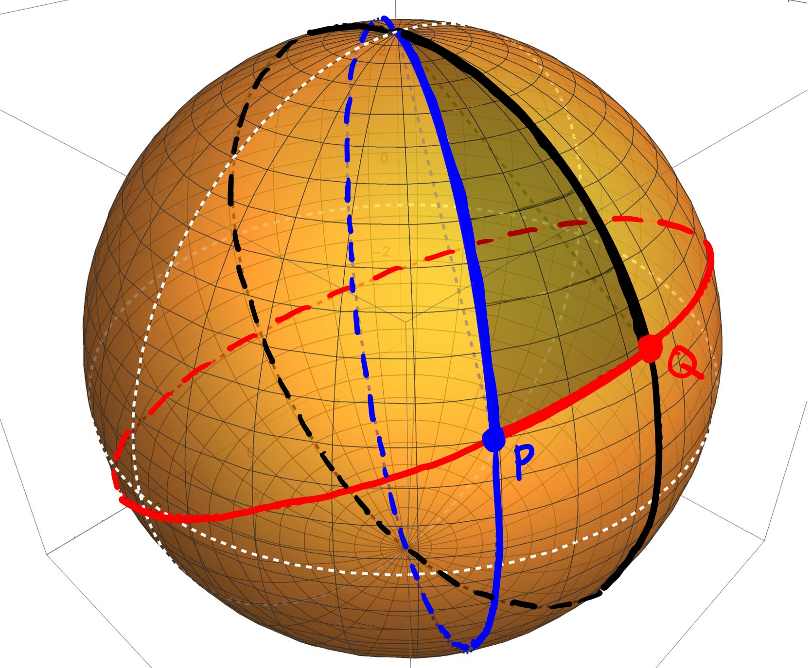
Figure 4: Examples of Geodesics on a Sphere: The Equator, All Lines of Longitude, and any Great Circle.

Outlining a Method to Find an Equation of a Great Circle

Here is one series of steps for obtaining a parametrically defined formula \(r(t)\) of a great circle on a sphere described by

\[\begin{align} r(\theta,\phi)&=(f(\phi)\cos(\theta),f(\phi)\sin(\theta),h(\phi)), \end{align}\] where \[\begin{align} f(\phi)=\rho\sin(\phi)\;\; \mbox{and}\;\; h(\phi)=\rho\cos(\phi): \end{align}\]

• For two latitude (\(\phi\)) and longitude (\(\theta\)) selections \(q=(\theta,\phi)\) and \(p=(\Theta,\Phi)\), find two distinct points of the sphere \(Q=r(q)=r(\theta,\phi)\) and \(P=r(p)=r(\Theta,\Phi)\).

• Find the vectors \(\overrightarrow{v}\) and \(\overrightarrow{w}\) from the center of the sphere (say the origin \(\cal{O}=(0,0,0)\)) defined by \[\begin{align} \overrightarrow{v}&=\overrightarrow{\cal{O}P}=P-\cal{O},\\ \overrightarrow{w}&=\overrightarrow{\cal{O}Q}=Q-\cal{O}. \end{align}\]

• A vector \(\overrightarrow{a}\) in the plane defined by \(\overrightarrow{v}\) and \(\overrightarrow{w}\) is of the form \(\overrightarrow{a}=\alpha \overrightarrow{v}+\beta \overrightarrow{w}\) (a linear combination). To find the coefficients \(\alpha\) and \(\beta\) of the linear combination, enforce the requirement that the vector \(\overrightarrow{a}\) be not only perpendicular to either vector \(\overrightarrow{v}\) or \(\overrightarrow{w}\) (choose \(\overrightarrow{w}\), and so \(\overrightarrow{a} \cdot \overrightarrow{w}=0\)), but also that \(\overrightarrow{a}\) is on the sphere (and so \(|\overrightarrow{a}|=\sqrt{\overrightarrow{a}\cdot \overrightarrow{a}}=\rho\)). This thought process gives two equations \[\begin{align} \overrightarrow{a} \cdot \overrightarrow{w}&=0\\ \sqrt{\overrightarrow{a}\cdot \overrightarrow{a}}&=\rho \end{align}\] which can be solved in Mathematica for the two unknowns \(\alpha\) and \(\beta\).

With \(\alpha\) and \(\beta\) so obtained, two perpendicular vectors, \(\overrightarrow{w}\) and \(\overrightarrow{a}=\alpha \overrightarrow{v}+\beta \overrightarrow{w}\) (both of length \(\rho\)) are known and the equation of the great circle containing the points \(P\) and \(Q\) is

\[\begin{align} r(t)&=\cos(t) \overrightarrow{a}+ \sin(t) \overrightarrow{w}, \end{align}\] where \(r(\pi/2)=Q\) and \(r(\#)=P\) (where \(\#\) can be obtained).

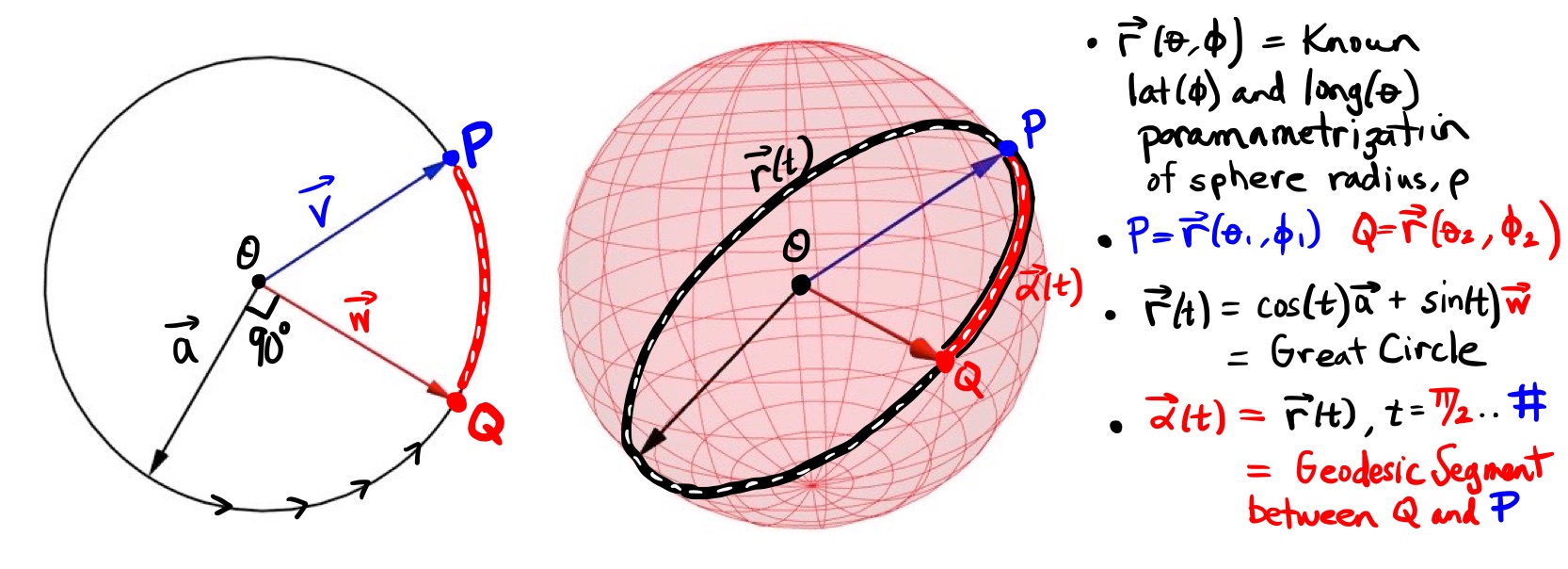
Figure 5: An Outline of a Method to Find the Equation of a Great Circle. The geodesic between two points \(P\) and \(Q\) on a sphere is the arc of a great circle connecting these two points (shown here is the shortest geodesic between the points).

Note: The equation of the Great Circle between two points \(P=r(\theta,\phi)\) and \(Q=r(\Theta,\Phi)\) on a sphere is detailed in the “Additional Resources” section of this post.

Here Then is a Geodesic Triangle…On the Earth

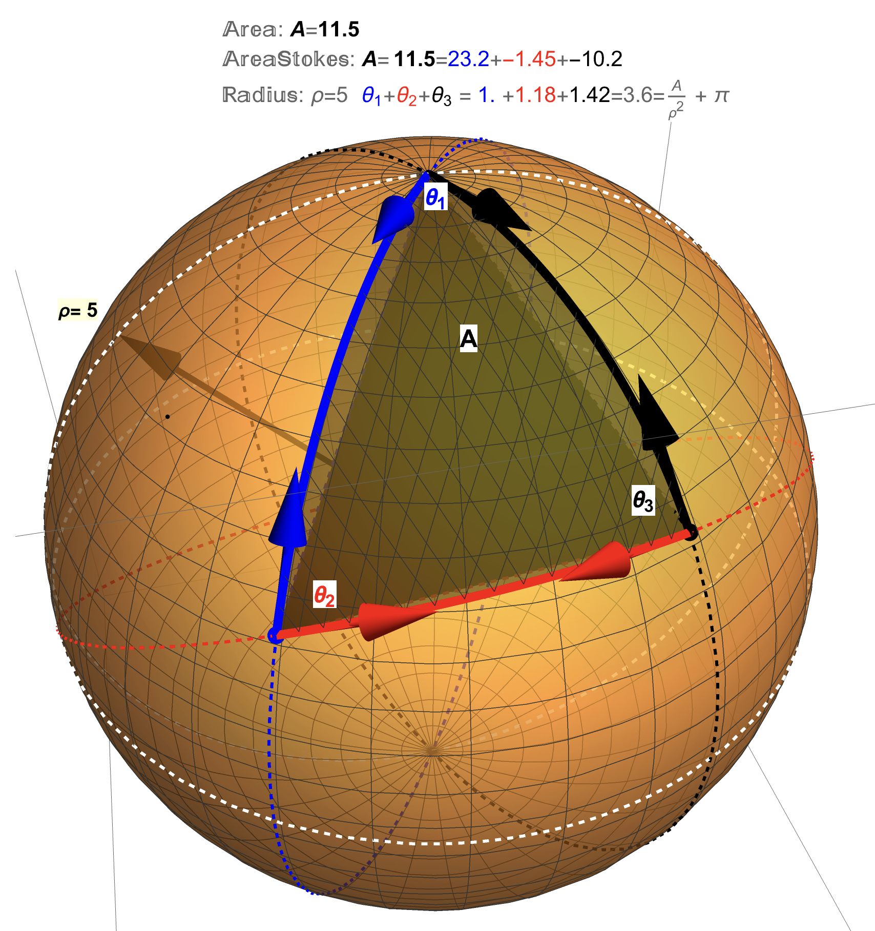
Figure 6: A Geodesic Triangle: The measure of the angles of this triangle (for example, \(\theta_{1}\)) can be found from the (tangent) vectors to the edges of the triangle (say, \(v_{1}\) and \(w_{1}\)) using the formula \(\theta_{1}=\mbox{arccos}\left(\frac{v_{1}\cdot w_{1}}{|v_{1}||w_{1}|}\right)\). The area of the geodesic triangle can be determined in a couple of ways (Stokes’s Theorem and Surface Area Integral) and will be discussed shortly.

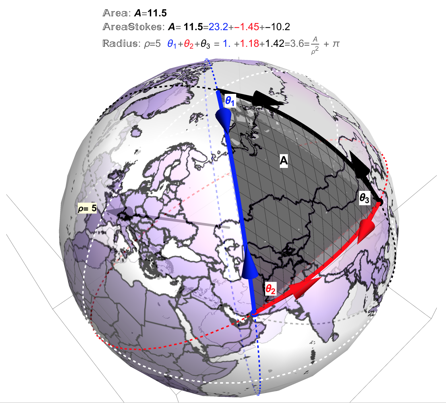
Figure 7: A Geodesic Triangle on the Earth.

The Big Result…A Euclidean Limit

In Figures 8 and 9 the relationship between the sum of angles of a geodesic triangle on a sphere of radius \(\rho\) with its area is shown to be, \[\begin{align} \Sigma_{i=1}^{3}\theta_{i}=\pi+\frac{A}{\rho^{2}}. \end{align}\]

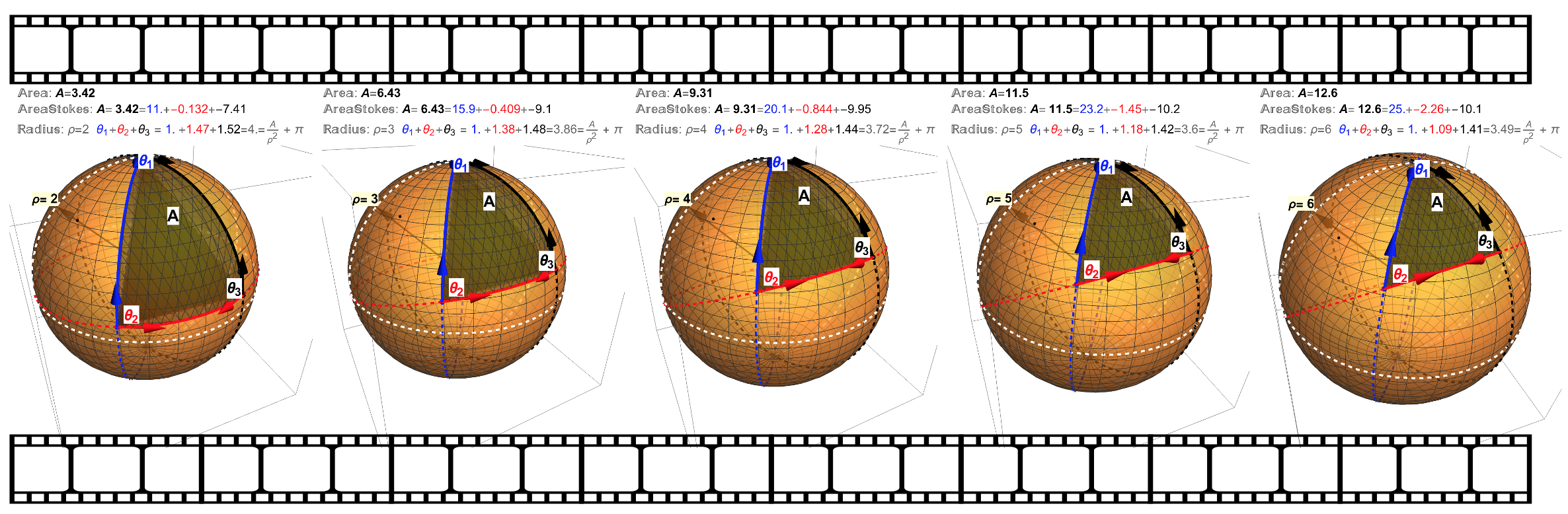
Figure 8: The Geodesic Triangles Star in a Film… As the radius \(\rho\) increases (progressing to the right in the film), the areas increase while the sum of the interior angles \(\theta_{1},\theta_{2}\) and \(\theta_{3}\) decrease. A natural question is what happens to the sum of angles as the radius continues to grow? Does the sum keep decreasing? Or does the sum approach some limit? It’s hard to tell in this film sequence as the sum of the angles are \(\Sigma_{i=1}^{3}\theta_{i}=4, 3.86, 3.72, 3.6\) and \(3.49\).

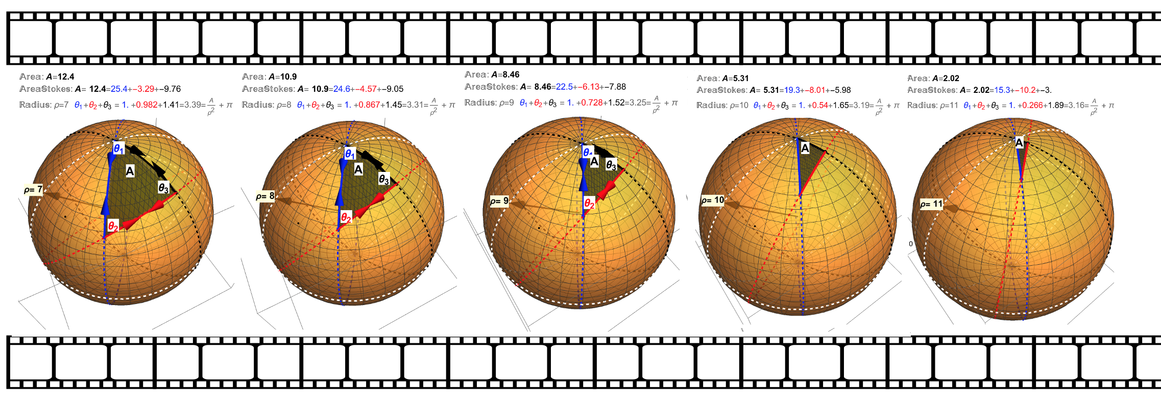
Figure 9: A Limit Appears…The sum of the angles for this segment of film are \(\Sigma_{i=1}^{3}\theta_{i}=3.39,3.31,3.25,3.19\), and \(3.16\). It turns out that each sum \(\Sigma_{i=1}^{3}\theta_{i}=\theta_{1}+\theta_{2}+\theta_{3}\) can also be obtained (without knowing each individual angle \(\theta_{i}\)) if one simply knows the geodesic triangle area and the radius of the sphere on which the triangle is drawn. That is, \(\Sigma_{i=1}^{3}\theta_{i}=\pi+\frac{A}{\rho^{2}}\). Note that the number \(\pi\) is about \(3.14\) which is the value the sum of angles approaches as the radius of the sphere continutes to grow.

From the Apple Book A Curvature Story we know that the curvature \(\kappa\) of a sphere of radius \(\rho\) is the constant \[\begin{align} \kappa=\frac{1}{\rho^{2}}, \end{align}\] from which it follows that \[\begin{align} \Sigma_{i=1}^{3}\theta_{i}=\pi+\kappa A. \end{align}\]

As the radius of the sphere increases (\(\rho \rightarrow \infty\)) then the curvature of the sphere decreases (\(\kappa \rightarrow 0\)) which means that, similar to the prior post The Cost of Curvature, the effects of curvature become negligable on the sum of the angles of a geodesic triangle. This is the Euclidean Limit: \[\begin{align} \Sigma_{i=1}^{3}\theta_{i}&=\pi+\frac{A}{\rho^{2}}=\pi+\kappa A \rightarrow \pi \\ &\mbox{as}\;\; \kappa \rightarrow 0 \;\; \mbox{(or}\;\; \rho \rightarrow \infty ). \end{align}\] That is, as the radius of the sphere increases then any geodesic triangle drawn on this sphere will look more and more like a normal (Euclidean) triangle whose angles are known to sum to \(\pi^{R}\) or \(180^{\circ}\) (see Figure 10 ).

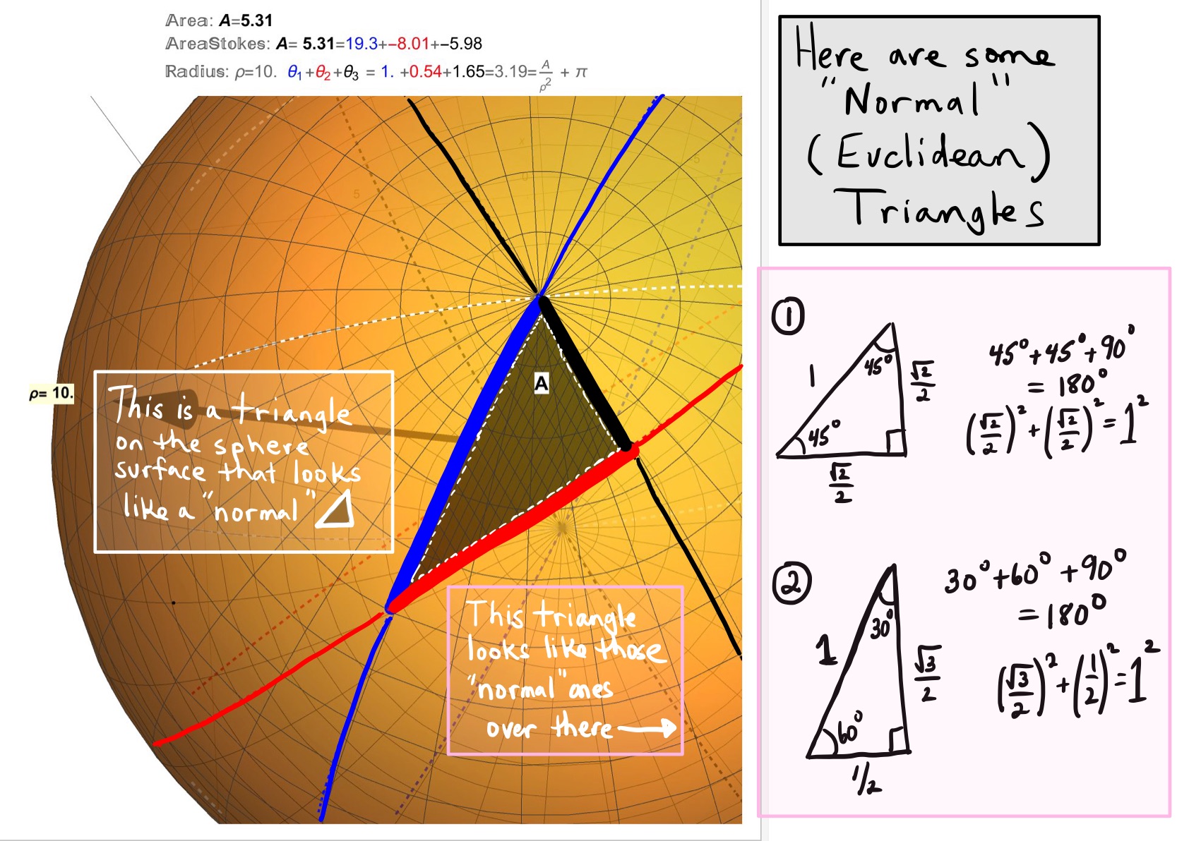
Figure 10: The Euclidean Limit: On a sphere of large radius, this triangle looks a lot like a “normal” (Euclidean) triangle. In a “normal” triangle, the angles add to \(\pi^{R}\) or \(180^{\circ}\) and the side lengths satisfy the Phythagorean Theorem \(a^{2}+b^{2}=c^{2}\).

Technical Difficulties in Computing Area…

In a first attempt at generating the images in this post I already knew the result \[\begin{align} \Sigma_{i=1}^{3}\theta_{i}=\pi+\frac{A}{\rho^{2}} \end{align}\] as a consequence of the Gauss-Bonnet Theorem (see Barrett Oneill, Elementary Differential Geometry, revised Second Edition, pg. 379).

I checked my code against this result in the case \(\rho=1\) and for a geodesic triangle whose edges were two lines of longitude and an arc of the equator (subtended by an angle of \(\theta=1\)). In this case the area of the region \(NPQ_{1}\) shown in Figure 11 is easy to compute using a Surface Area Integral \[\begin{align} A=\int_{\phi=0}^{\phi=\pi/2} \int_{\theta=0}^{\theta=1} \sin(\phi)\; d\theta\;d\phi=1. \end{align}\]

This area computation is corroborated since the sum of angles in the \(\rho=1\),\(\theta_{1}=1\)-case seen in Figure 11 evaluates to \(4.14\). Consequently, \[\begin{align} \Sigma_{i=1}^{3}\theta_{i}&=\pi+\frac{A}{1^{2}}=\pi+A=4.14 \\ &\implies A=4.14-\pi=1. \end{align}\]

Anticipating a time when I would need to compute the area of a region \(NPQ_{2}\) as shown in Figure 11, I double checked this area computation using Stoke’s Theorem. While this approach did correctly compute the area in this case, the line integrals of Stoke’s Theorem along the edges of the geodesic triangle are problematic computationally (from a time expense point of view) since the edge between the two points \(P\) and \(Q_{2}\) was parameterized by \(r(t)=\cos(t)\overrightarrow{v}+\sin(t)\overrightarrow{Q_{2}}\). Recall from a previous section Outlining a Method to Find an Equation of a Great Circle that in this parameterization \(\overrightarrow{v}\) is a vector in the plane defined by \({\overrightarrow P}\) and \(\overrightarrow{Q_{2}}\) and that the values of the parameter are \(t=\pi/2 ... \#\) for some computationally not-nice value \(\#\).

Note: The details behind using Stoke’s Theorem (three line integrals on the boundary curves) to evaluate the area of a geodesic triangle can be found in the “Additional Resources” section of this post.

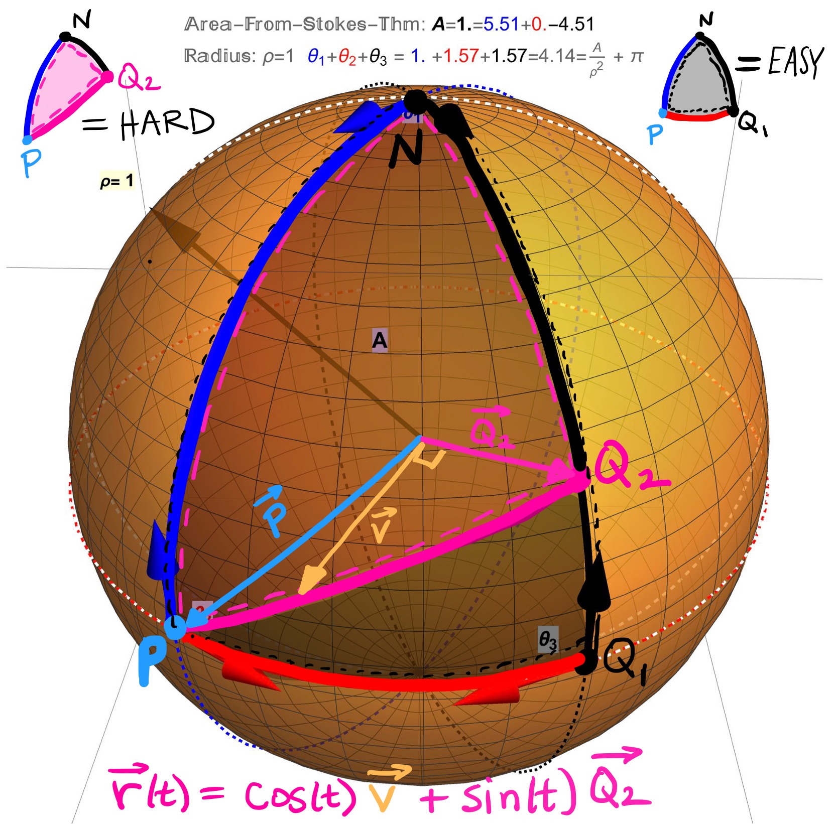
Figure 11: Computational Complexity: Computing area of a geodesic triangle with one edge being the great circle between the two points \(P\) and \(Q_{2}\) parameterized by \(r(t)=\cos(t)\overrightarrow{v}+\sin(t)\overrightarrow{Q_{2}}\) is computationally intensive for a couple of reasons, not least of which being that the upper parameter \(\#\) of the interval \(t=\pi/2 ... \#\) is a not-nice number involving an inverse trig function. For these parametrization reasons, we go back to the drawing board to come up with a better method for describing and computing the area of a geodesic triangle.

Back to the Drawing Board…Simplify to Lines

While I was able to use Stoke’s Theorem to compute the area the region \(NPQ_{1}\) in Figure 11, the theorem was prohibitively slow for the region \(NPQ_{2}\). I spent some time trying to describe a region like \(NPQ_{2}\) in spherical coordinates, and therefore avoid Stoke’s Therorem altogether, by evaluating a Surface Area Integral \[\begin{align} \int_{\theta=0}^{\theta=1} \int_{\phi=0}^{\phi=\phi(\theta)} \rho^{2}\sin(\phi)\;d\phi \; d\theta, \end{align}\] but was unable to find a requisite function \(\phi(\theta)\). The solution to several problems is to describe a region like \(NPQ_{2}\) using lines instead. The idea, illustrated in Figure 12, is simply to stretch/scale each vector on the flat triangular plane containing the vertices of geodesic triangle by the appropriate amount to reach the sphere’s surface. Thanks to Professor Bill Cook for general conversations about this post and this suggestion in particular. This process can be outlined as

• Take the three corners of the geodesic triangle, \(P=r(\theta_{1},\phi_{1})\), \(Q=r(\theta_{2},\phi_{2})\), and \(R=r(\theta_{3},\phi_{3})\) and find the equations of the straight lines between them using the vectors between these points. For example, the vector between the points \(P\) and \(Q\) is \(\overrightarrow{PQ}=Q-P\) and therefore the line between these points is \(l(t)=P+\overrightarrow{PQ}\cdot t\) with values of a new parameter \(t\) ranging from \(t=0\) to \(t=1\) since \(l(0)=P\) and \(l(1)=P+(Q-P)\cdot 1=Q\).

• Consider a point \(A\) on the line \(l(t)\). The vector \(\overrightarrow{A}=\overrightarrow{\cal{O}A}=A-\cal{O}\) to this point \(A\) has some length \(|\overrightarrow{A}|\) and therefore the vector \(\overrightarrow{A}/|\overrightarrow{A}|\) has length 1. It follows that \(\rho\cdot \frac{\overrightarrow{A}}{|\overrightarrow{A}|}\) has length \(\rho\) (the radius of the desired sphere) and therefore is a vector on the sphere.

• The edge of the geodesic triangle between the points \(P\) and \(Q\) can then be found by stretching each vector on the line \(l(t)\) to a new curved line \(L(t)=\rho \frac{\overrightarrow{l(t)}}{|\overrightarrow{l(t)}|}\). The same can be done for the other two edges. This type of parameterization of the edges is much quicker computationally for use with Stoke’s Theorem should one want to keep going down that track for computing area.

• To avoid Stoke’s Theorem altogether, we can simply find an equation of the plane (given by the black triangle in Figure 11) and stretch this to the surface of the sphere. The equation of this plane given parameterically is, for example,

\[\begin{align} l(t,s)&=P+\overrightarrow{PQ}\cdot t+\overrightarrow{PR}\cdot s\\ &= P+(Q-P)\cdot t + (R-P)\cdot s\\ &= P-Pt-Ps+Qt+Rs \\ &=(1-t-s)P+Qt+Rs. \end{align}\]

• Therefore the region enclosed by a geodesic triangle with vertices \(P,Q\) and \(R\) is \[\begin{align} r(t,s)=\rho \cdot \frac{l(t,s)}{|l(t,s)|}, \end{align}\] where the values of the parameters are \(t=0 \ldots 1\) and \(s=0\ldots 1-t\) since \(r(t=0,s=0)=P\), \(r(t=1,s=0)=Q\), and \(r(t=0,s=1)=R\).

Finally, the area of a the geodesic triangle can be obtained from a Surface Area Integral \[\begin{align} \int_{t=0}^{t=1} \int_{s=0}^{s=1-t} \left|\frac{\partial r}{\partial t} \times \frac{\partial r}{\partial s}\right| \; ds \;dt . \end{align}\]

As can be seen in Figure 12, both Stoke’s Theorem (along the edges of the geodesic triangle parameterized as stretched lines) and the surface area integral (geodesic triangle parameterized as a stretched triangular plane) give the same values. It is these “stretchy” parameterizations we used in all of the figures in this post.

Note: The formulas for Great Circles (in two parameterizations) and the some details behind Stoke’s Theorem will appear in the “Additional Resources” section of this post.

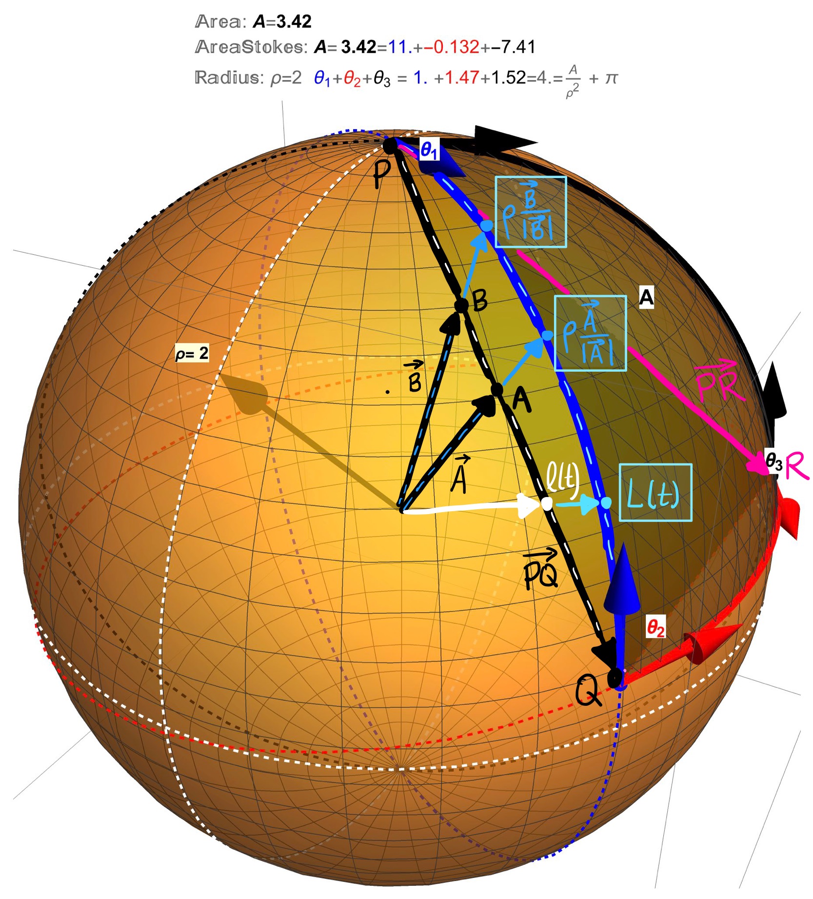
Figure 12: A Stretchy Idea: (1) The vector between the points \(P\) and \(Q\) is \(\overrightarrow{PQ}=Q-P\) and therefore the line between these points is \(l(t)=P+\overrightarrow{PQ}\cdot t\) with values of a new parameter \(t\) ranging from \(t=0\) to \(t=1\). (2) Pick a point \(A\) on the line \(l(t)\). The vector \(\overrightarrow{A}=\overrightarrow{\cal{O}A}=A-\cal{O}\) to this point \(A\) has some length \(|\overrightarrow{A}|\) and therefore the vector \(\overrightarrow{A}/|\overrightarrow{A}|\) has length 1. It follows that \(\rho\cdot \frac{\overrightarrow{A}}{|\overrightarrow{A}|}\) has length \(\rho\) (the radius of the desired sphere) and therefore is a vector on the sphere. (3) The edge of the geodesic triangle between the points \(P\) and \(Q\) can then be found by stretching each vector on the line \(l(t)\) to a new curved line \(L(t)=\rho \frac{\overrightarrow{l(t)}}{|\overrightarrow{l(t)}|}\). (4) The equation of the plane is \(l(t,s)=(1-t-s)P+Qt+Rs\) and therefore the region enclosed by the geodesic triangle can be described parametrically as \(r(t,s)=\rho \cdot \frac{l(t,s)}{|l(t,s)|}\) where \(t=0\ldots 1\) and \(s=0 \ldots 1-t\).

A Hint at Some Technical Details Following From the Sphere Being a Surface of Revolution…

In Figure 4, examples of geodesics on a sphere were shown without first giving a definition of a geodesic. The reason for this omission is simply that a formal definition requires a lot mathematical and symbological machinery. Rather than continuing to omit these details, I will try to summarize some of the technical issues as these tools and techniques will appear in future posts.

• Kernel-Index Notation, Numbering, and Naming Rather than write the sphere as a parameterized surface of revolution in the notation \[\begin{align} r(\theta,\phi)=(f(\phi) \cos (\theta) , f(\phi) \sin (\theta), h(\phi)) \end{align}\] where \[\begin{align} f(\phi)=\rho\sin(\phi)\;\; \mbox{and}\;\; h(\phi)=\rho\cos(\phi). \end{align}\] we will write the sphere equivalently as a vector-valued function in kernel-index notation \[\begin{align} F^{i}(q^{\alpha})=\begin{pmatrix} f(\phi) \cos (\theta) \\ f(\phi) \sin (\theta) \\ h(\phi) \end{pmatrix}, \end{align}\] with coordinate vector \[\begin{align} q^{\alpha}=\begin{pmatrix} \theta \\ \phi \end{pmatrix} \end{align}\] and \[\begin{align} f(\phi)=\rho\sin(\phi)\;\; \mbox{and}\;\; h(\phi)=\rho\cos(\phi). \end{align}\] This is the kernel-index notation: \[\begin{align} F^{i}:& \;\;\mbox{the symbol}\;\; F \;\; \mbox{is the kernel and} \\ &\;\;\mbox{and the symbol} \;\; i \;\; \mbox{is the row index}\\ &\;\;\mbox{which runs i=1,2,3}\\ &\\ q^{\alpha}:& \;\; q \;\; \mbox{the kernel} \;\; \alpha \;\; \mbox{the row index}\\ \; &\;\;\mbox{which runs $\alpha$=1,2}\\ \end{align}\] The upper index \(i\) refers to the ith-row of the vector \(F^{i}\) and the upper \(\alpha\) index refers to the \(\alpha\)th-row of the vector \(q^{\alpha}\). For example, the 1st (row) entry of the vector \(q^{\alpha}\) is \(q^{1}=\theta\) with 2nd (row) entry \(q^{2}=\phi\) while the 1st (row) entry of the vector \(F^{i}\) (also called the x-component of the vector \(\Psi^{i}\)) is \(x=F^{1}=f(\phi)\cos(\theta)\). The vector \(q^{\alpha}\) is called the coordinate vector with first coordinate \(q^{1}=\theta\) and second coordinate \(q^{2}=\phi\).

• Coordinate Curves and Their Mappings to a Surface. If the coordinates change with a parameter (say time, t) then a curve in the coordinate space (a coordinate curve) can be written as \(q^{\alpha}(t)\) and two vectors can be obtained by differentiation \(\dot{q}^{\alpha}(t)\) (the coordinate velocity vector) and \(\ddot{q}^{\alpha}(t)\) (the coordinate acceleration vector) \[\begin{align} q^{\alpha}(t)=\left(\begin{array}{l} \theta(t) \\ \phi(t) \end{array}\right),\dot{q}^{\alpha}=\left(\begin{array}{l} \theta_{t} \\ \phi_{t} \end{array}\right), \ddot{q}^{\alpha}=\left(\begin{array}{l} \theta_{t, t} \\ \phi_{t, t} \end{array}\right) \end{align}\] where, for example \(\phi_{t}=d\phi/dt\) is the first derivative of \(\phi\) with respect to \(t\) and \(\theta_{t,t}=d^{2}\theta/dt^{2}\) is the second time derivative of \(\theta\). For example, in coordinates, the Equator is a line \[\begin{align} q^{\alpha}(t)&=\left(\begin{array}{l} \theta(t) \\ \phi(t) \end{array}\right)=\left(\begin{array}{l} t \\ \pi/2 \end{array}\right) \;\; \mbox{for}\;\; t=0\ldots 2\pi \\ \dot{q}^{\alpha}&=\left(\begin{array}{l} \theta_{t} \\ \phi_{t} \end{array}\right)=\left(\begin{array}{l} 1 \\ 0 \end{array}\right), \end{align}\] and the Prime Meridian, in coordinates, is also a line \[\begin{align} q^{\alpha}(t)&=\left(\begin{array}{l} \theta(t) \\ \phi(t) \end{array}\right)=\left(\begin{array}{l} 0 \\ t \end{array}\right) \;\; \mbox{for} \;\; t=0\ldots 2\pi\\ \dot{q}^{\alpha}&=\left(\begin{array}{l} \theta_{t} \\ \phi_{t} \end{array}\right)=\left(\begin{array}{l} 0 \\ 1 \end{array}\right). \end{align}\] In both cases (the Equator and Prime Meridian) the coordinate acceleration vector is \[\begin{align} \ddot{q}^{\alpha}=\left(\begin{array}{l} \theta_{t,t} \\ \phi_{t,t} \end{array}\right)=\left(\begin{array}{l} 0 \\ 0 \end{array}\right). \end{align}\] The coordinate curves \(q^{\alpha}(t)\) are mapped (or drawn) onto the surface by applying the vector function \(F^{i}\) to \(q^{\alpha}(t)\) as \(F^{i}(q^{\alpha}(t))\). For example, the Equator maps to the surface according to \[\begin{align} F^{i}(q^{\alpha}(t))&=\begin{pmatrix} \cos (\theta)\sin(\phi) \\ \sin (\theta)\sin(\phi) \\ \cos(\phi) \end{pmatrix}\biggr \rvert_{\theta=t,\phi=\pi/2}\\ &=\begin{pmatrix} \cos (t) \\ \sin (t) \\ 0 \end{pmatrix}, \end{align}\] while the Prime Meridian maps as \[\begin{align} F^{i}(q^{\alpha}(t))&=\begin{pmatrix} \cos (\theta)\sin(\phi) \\ \sin (\theta)\sin(\phi) \\ \cos(\phi) \end{pmatrix}\biggr \rvert_{\theta=t,\phi=\pi/2}\\ &=\begin{pmatrix} \sin(t) \\ 0 \\ \cos(t) \end{pmatrix}. \end{align}\] These mappings can be seen in Figures 13 and Figures 14

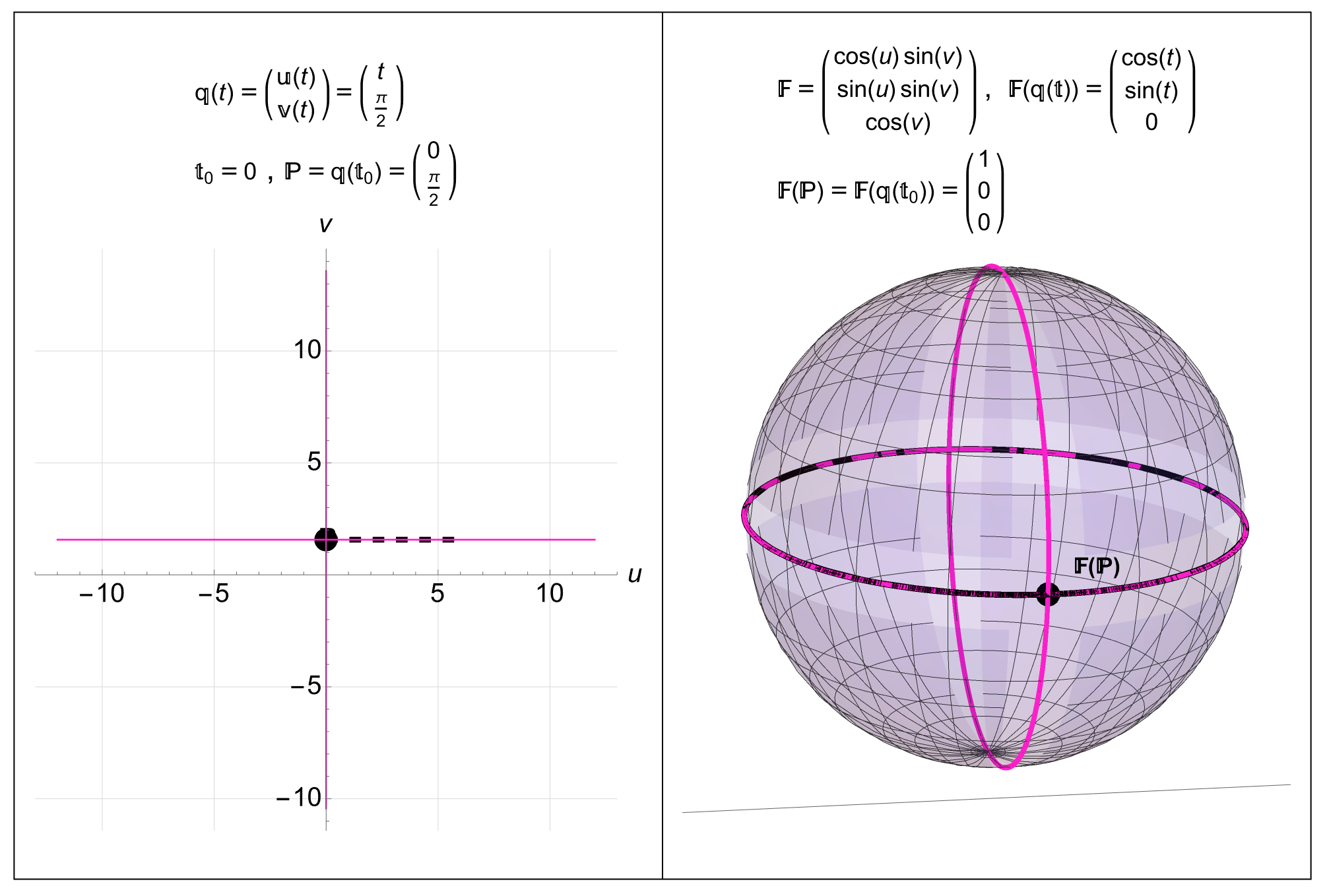
Figure 13: Mapping the Equator in Coordinate Space to Real 3D Space: A point \(P=(0,\pi/2)\) in 2D coordinate space maps to the point \(F^{i}(P)=(1,0,0)\) in 3D space. The black line \(q^{\alpha}(t)=(t,\pi/2)\) in coordinate space goes through the point \(P\) at time \(t=0\) and maps to the black curve in 3D space \(F^{i}(q^{\alpha}(t))=(\cos(t),\sin(t),0)\) (the Equator). We are also seeing the two pink coordinate lines through \(P\) mapped onto the surface as the two pink curves.

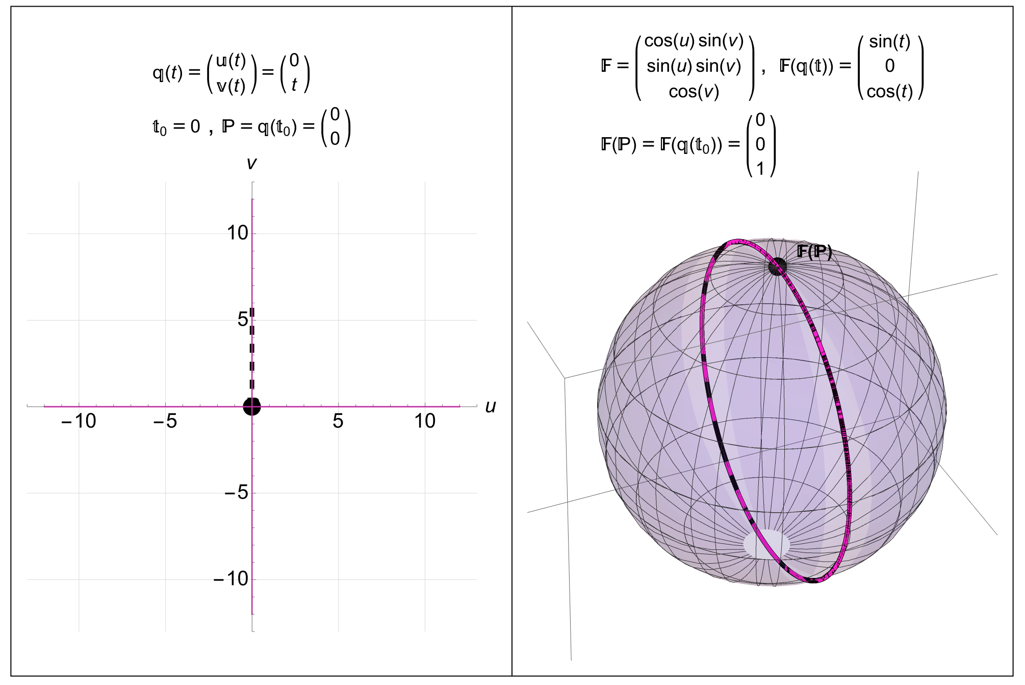
Figure 14: Mapping the Prime Meridian in Coordinate Space to Real 3D Space: A point \(P=(0,0)\) in 2D coordinate space maps to the point \(F^{i}(P)=(0,0,1)\) in 3D space. The black line \(q^{\alpha}(t)=(t,\pi/2)\) in coordinate space goes through the point \(P\) at time \(t=0\) and maps to the black curve in 3D space \(F^{i}(q^{\alpha}(t))=(\cos(t),\sin(t),0)\) (the Prime Meridian). We are also seeing the two pink coordinate lines through \(P\) mapped onto the surface as the two pink curves (one of the pink curves is a single point at the North Pole.

The Geometry of the Sphere as a Surface of Revolution

In future posts we will explain in detail the geometric computations of and the meaning of each of the geometric objects shown below. These computations were done using a Maple package I wrote called tensorAddOns. Our goal here to record this data and use what we need to define the geodesic equations on a surface of revolution with specfic application to a sphere.

• Surface of Revolution with Jacobian and Hessian: \[\begin{align} &F^{i}(q^{\alpha})=\begin{pmatrix} f(\phi) \cos (\theta) \\ f(\phi) \sin (\theta) \\ h(\phi) \end{pmatrix} \;\; \mbox{with}\;\; q^{\alpha}=\begin{pmatrix} \theta \\ \phi \end{pmatrix}, \\ &F^{i}_{,\alpha}=\frac{\partial F^{i}}{\partial q^{\alpha}}=\left(\begin{array}{cc} -f(\phi) \sin (\theta) & \left(f_{\phi}\right) \cos (\theta) \\ f(\phi) \cos (\theta) & \left(f_{\phi}\right) \sin (\theta) \\ 0 & h_{\phi} \end{array}\right), \\ &F^{i}_{, \alpha \beta}=\frac{\partial^{2} F^{i}}{\partial q^{\alpha} \partial q^{\beta}}=\left(\begin{array}{c} {\left(\begin{array}{cc} -f(\phi) \cos (\theta) & -\left(f_{\phi}\right) \sin (\theta) \\ -\left(f_{\phi}\right) \sin (\theta) & \left(f_{\phi, \phi}\right) \cos (\theta) \end{array}\right)} \\ {\left(\begin{array}{cc} -f(\phi) \sin (\theta) & \left(f_{\phi}\right) \cos (\theta) \\ \left(f_{\phi}\right) \cos (\theta) & \left(f_{\phi, \phi}\right) \sin (\theta) \end{array}\right)} \\ {\left(\begin{array}{cc} 0 & 0 \\ 0 & h_{\phi, \phi} \end{array}\right)} \end{array}\right) \end{align}\]

• Metric Tensors (First Fundamental Form) of a Surface of Revolution: \[\begin{align} g_{\alpha\beta}&=\left(\begin{array}{cc} f(\phi)^{2} & 0 \\ 0 & \left(f_{\phi}\right)^{2}+\left(h_{\phi}\right)^{2} \end{array}\right) \\ g^{\alpha\beta}&=\left(\begin{array}{cc} \frac{1}{f(\phi)^{2}} & 0 \\ 0 & \frac{1}{\left(f_{\phi}\right)^{2}+\left(h_{\phi}\right)^{2}} \end{array}\right) \end{align}\]

• Normal Vector to a Surface of Revolution: \[\begin{align} u_{i}=\left(\frac{\cos (\theta)\left(h_{\phi}\right)}{d(\phi)} \frac{\sin (\theta)\left(h_{\phi}\right)}{d(\phi)}-\frac{f_{\phi}}{d(\phi)}\right) \end{align}\] where the denominator function is \[\begin{align} d(\phi)=\sqrt{\left(f_{\phi}\right)^{2}+\left(h_{\phi}\right)^{2}}. \end{align}\]

• Second Fundamental Form of a Surface of Revolution: \[\begin{align} b_{\alpha\beta}&=u_{i}F_{,\alpha\beta}^{i}\\ &=\left(\begin{array}{cc} -\frac{f(\phi)\left(h_{\phi}\right)}{\sqrt{\left(f_{\phi}\right)^{2}+\left(h_{\phi}\right)^{2}}} & 0 \\ 0 & \frac{-\left(f_{\phi}\right)\left(h_{\phi, \phi}\right)+\left(h_{\phi}\right)\left(f_{\phi, \phi}\right)}{\sqrt{\left(f_{\phi}\right)^{2}+\left(h_{\phi}\right)^{2}}} \end{array}\right) \end{align}\]

• Shape Operator of a Surface of Revolution: \[\begin{align} b_{\alpha}^{\beta}&=g^{\sigma \beta} b_{\alpha \sigma}\\ &=\left(\begin{array}{cc} -\frac{h_{\phi}}{f(\phi) \sqrt{\left(f_{\phi}\right)^{2}+\left(h_{\phi}\right)^{2}}} & 0 \\ 0 & \frac{-\left(f_{\phi}\right)\left(h_{\phi, \phi}\right)+\left(h_{\phi}\right)\left(f_{\phi, \phi}\right)}{\left(\left(f_{\phi}\right)^{2}+\left(h_{\phi}\right)^{2}\right)^{3 / 2}} \end{array}\right) \end{align}\]

• Christoffel Symbols a Surface of Revolution, \(\Gamma_{\alpha \beta}^{\sigma}=\frac{1}{2} g^{\sigma \kappa}\left(g_{\{\alpha \beta, \kappa\}}\right)=\frac{1}{2} g^{\sigma \kappa}\left(-g_{\alpha \beta, \kappa}+g_{\beta \kappa, \alpha}+g_{\kappa \alpha, \beta}\right)\) displayed here as a vector of symmetric matrices (with the upper index \(\sigma\) the vector index) \[\begin{align} \Gamma^{\sigma}_{\alpha \beta}=\left( \begin{gathered} \left(\begin{array}{cc} 0 & \frac{f_{\phi}}{f(\phi)} \\ \frac{f_{\phi}}{f(\phi)} & 0 \end{array}\right)\\ \left(\begin{array}{cc} -\frac{\left(f_{\phi}\right) f(\phi)}{\left(f_{\phi}\right)^{2}+\left(h_{\phi}\right)^{2}} & 0 \\ 0 & \frac{\left(f_{\phi}\right)\left(f_{\phi, \phi}\right)+\left(h_{\phi}\right)\left(h_{\phi, \phi}\right)}{\left(f_{\phi}\right)^{2}+\left(h_{\phi}\right)^{2}} \end{array}\right) \end{gathered}\right). \end{align}\]

• The (lowered) Riemann Curvature Tensor a Surface of Revolution, \(R_{\alpha \beta \rho \eta}=g_{\sigma \eta}\left(\Gamma_{[\alpha|\rho|, \beta]}^{\sigma}+\Gamma_{[\alpha|\rho|}^{\kappa} \cdot \Gamma_{\beta] \kappa}^{\sigma}\right)\) displayed here as a matrix (indexed by \(\rho\) and \(\eta\)) of anti-symmetric matrices (indexed by \(\alpha\) and \(\beta\))

\[\begin{align} R_{\alpha \beta \rho \eta}=\begin{pmatrix} \begin{pmatrix} 0 & 0 \\ 0 & 0 \end{pmatrix} & \begin{pmatrix} 0 & R_{1212} \\ -R_{1212} & 0 \end{pmatrix}\\ \begin{pmatrix} 0 & -R_{1212} \\ R_{1212} & 0 \end{pmatrix} & \begin{pmatrix} 0 & 0 \\ 0 & 0 \end{pmatrix} \end{pmatrix}, \end{align}\]

where \[\begin{align} R_{1212}&=\operatorname{det}\left(b_{\alpha \beta}\right)\\ &=-\frac{f(\phi)\left(h_{\phi}\right)\left(-\left(f_{\phi}\right)\left(h_{\phi, \phi}\right)+\left(h_{\phi}\right)\left(f_{\phi, \phi}\right)\right)}{\left(f_{\phi}\right)^{2}+\left(h_{\phi}\right)^{2}}. \end{align}\]

• Gauss Curvature of Surface of Revolution, \(K=R_{1212}/det(g_{\alpha\beta})\):

\[\begin{align} K=-\frac{\left(h_{\phi}\right)\left(-\left(f_{\phi}\right)\left(h_{\phi, \phi}\right)+\left(h_{\phi}\right)\left(f_{\phi, \phi}\right)\right)}{f(\phi)\left(\left(f_{\phi}\right)^{2}+\left(h_{\phi}\right)^{2}\right)^{2}} \end{align}\]

• The Geodesic Equations on a Surface of Revolution: \(\ddot{q}^{\sigma}+\Gamma_{\alpha \beta}^{\sigma}\dot{q}^{\alpha}\dot{q}^{\beta}=0\)

\[\begin{align} &\theta_{t, t}+\left(\frac{2f_{\phi}}{f(\phi)}\right)\phi_{t}\theta_{t}=0,\\ &\phi_{t, t}+\mathbb{A}(\phi)\cdot \left(\phi_{t}\right)^{2}-\mathbb{B}(\phi)\cdot \left(\theta_{t}\right)^{2}=0, \end{align}\] where

\[\begin{align} \mathbb{A}(\phi)&= \left(\frac{\left(h_{\phi}\right)\left(h_{\phi, \phi}\right)}{\left(f_{\phi}\right)^{2}+\left(h_{\phi}\right)^{2}}+\frac{\left(f_{\phi}\right)\left(f_{\phi, \phi}\right)}{\left(f_{\phi}\right)^{2}+\left(h_{\phi}\right)^{2}}\right), \end{align}\] and \[\begin{align} \mathbb{B}(\phi)\left(\frac{\left(f_{\phi}\right) f(\phi)}{\left(f_{\phi}\right)^{2}+\left(h_{\phi}\right)^{2}}\right). \end{align}\]

As a demonstration of the tensorAddOns package I wrote in Maple (and a more specific instance of the geometric formulas above), we show screenshots of the calling sequence and output of the code in the case of a sphere. A sphere is surface of revolution \[\begin{align} F^{i}(q^{\alpha})=\begin{pmatrix} f(\phi) \cos (\theta) \\ f(\phi) \sin (\theta) \\ h(\phi) \end{pmatrix}, \end{align}\] with functions \(f(\phi)=\rho\sin(\phi)\) and \(h(\phi)=\rho\cos(\phi)\).

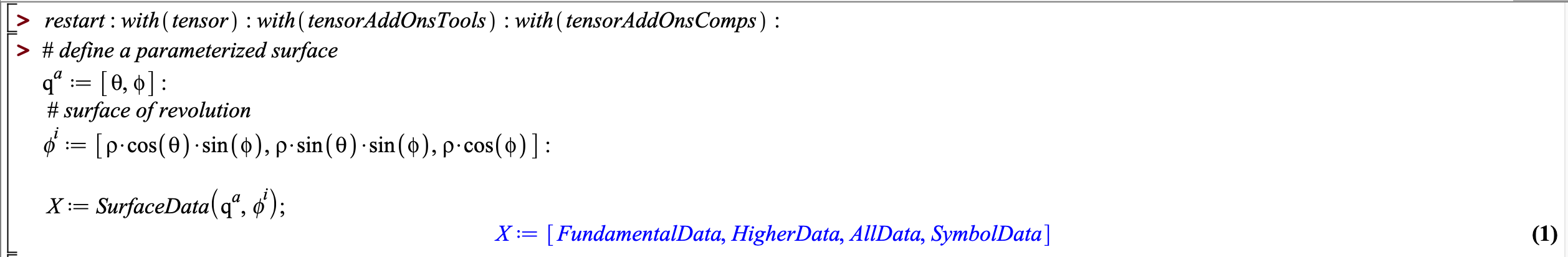
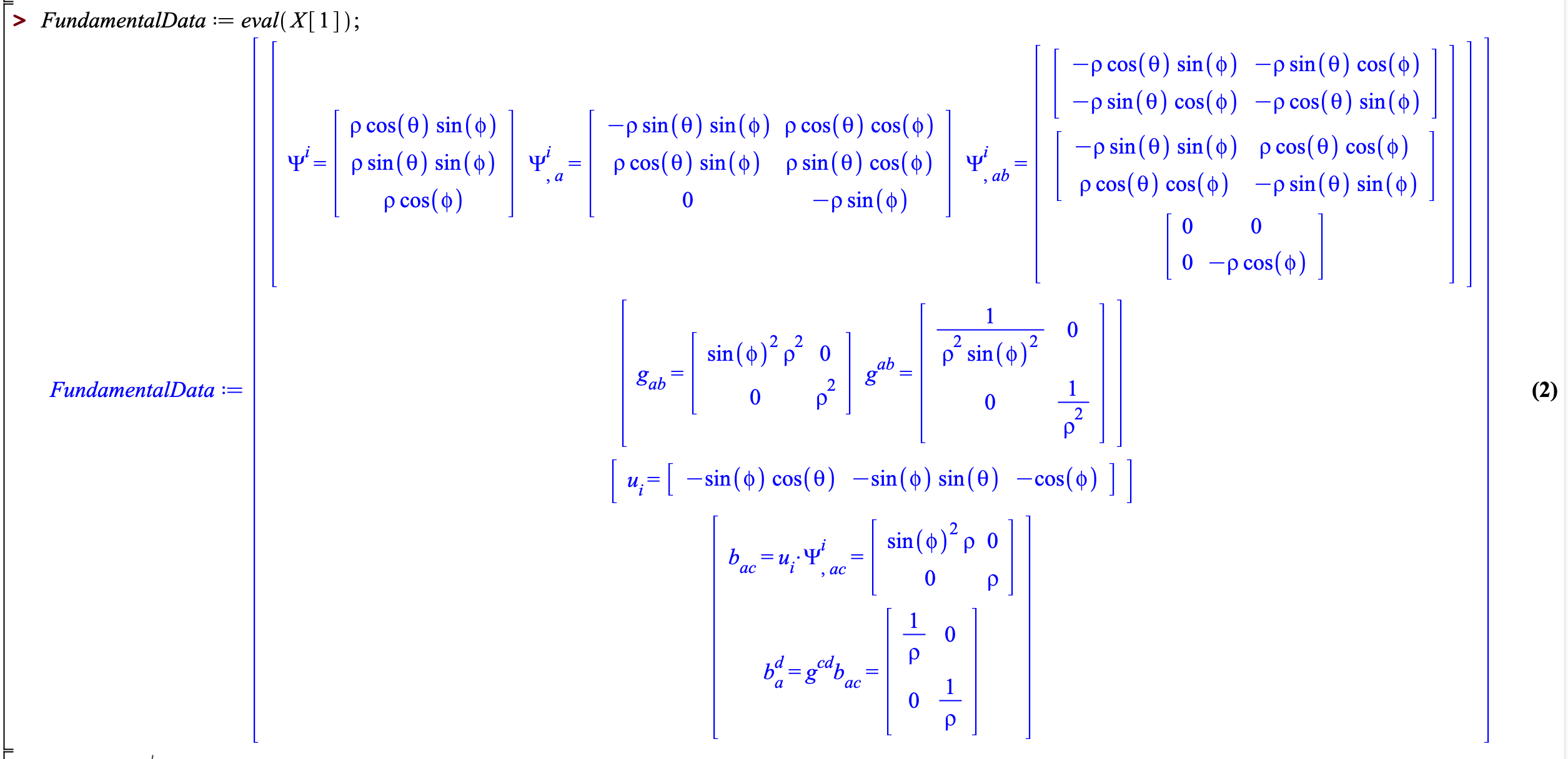
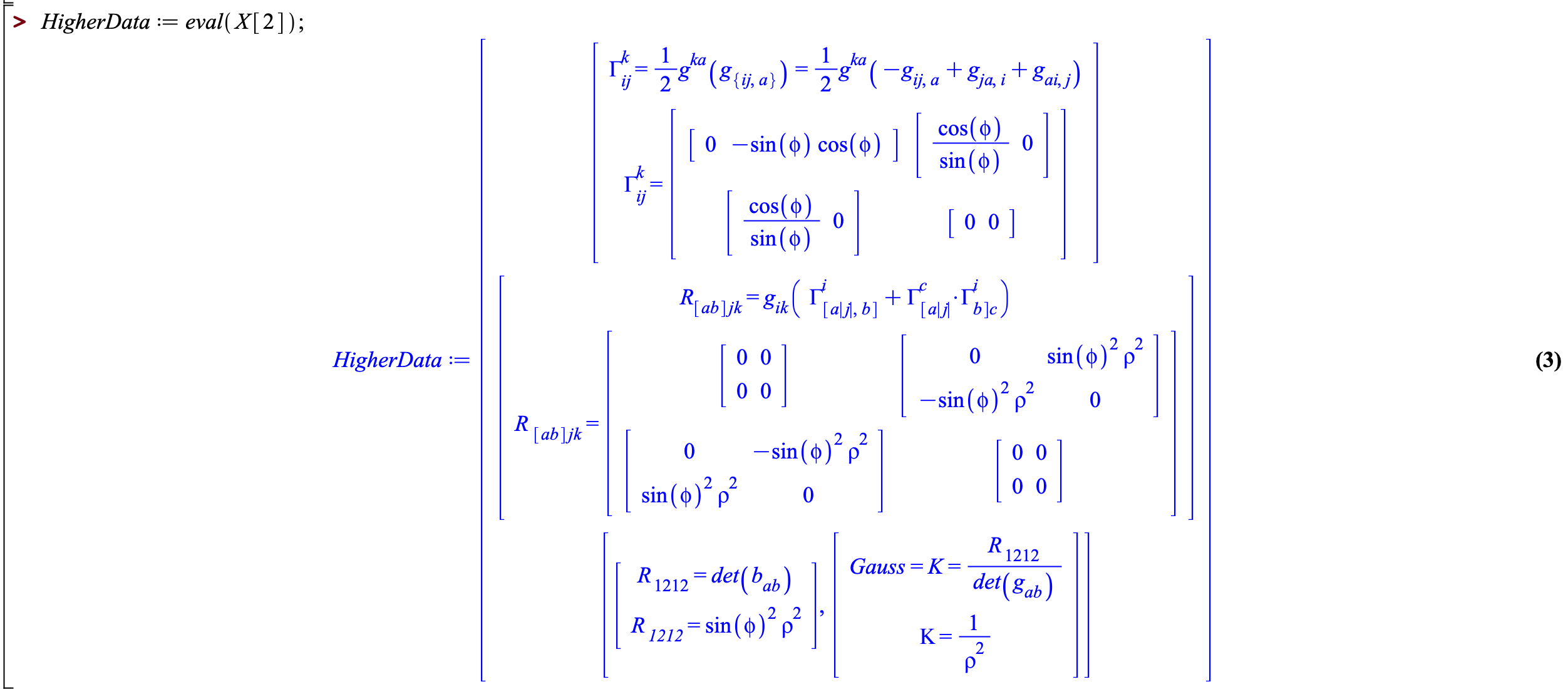
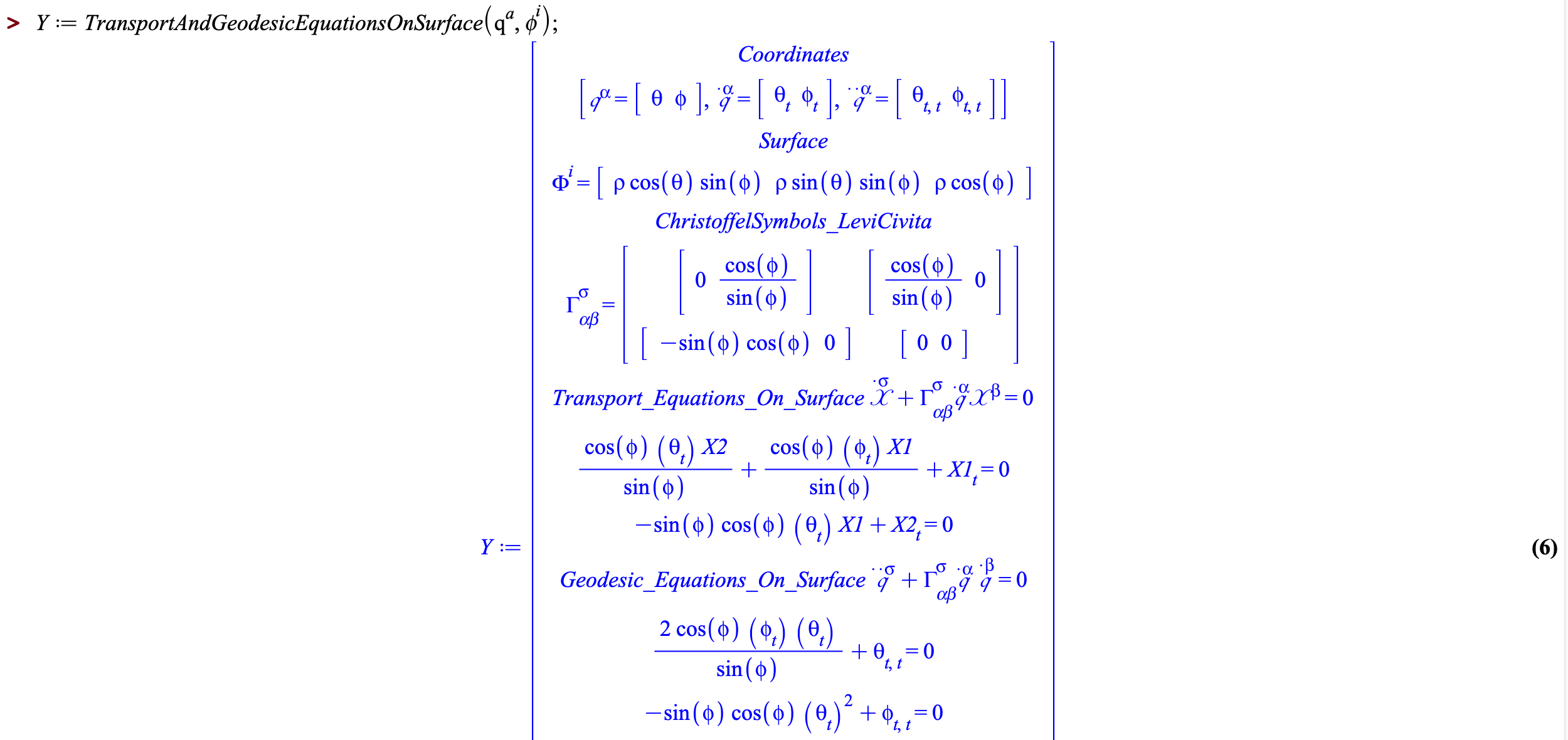
Figure 15: Calling sequence and output of Maple package tensorAddOns: Surface Data and Geodesic Equations on a Sphere.

Special Coordinate Curves Called Geodesics: On a Sphere

From the computations in Section The Geometry of the Sphere as a Surface of Revolution we see that in the parameterization of the sphere \[\begin{align} F^{i}(q^{\alpha})=\begin{pmatrix} \rho\cos (\theta)\sin(\phi) \\ \rho\sin (\theta)\sin(\phi) \\ \rho\cos(\phi) \end{pmatrix} \;\; \mbox{where} \;\; q^{\alpha}=\begin{pmatrix} \theta \\ \phi \end{pmatrix}, \end{align}\] with coordinate velocity vector and coordinate acceleration vector \[\begin{align} q^{\alpha}(t)=\left(\begin{array}{l} \theta(t) \\ \phi(t) \end{array}\right),\dot{q}^{\alpha}=\left(\begin{array}{l} \theta_{t} \\ \phi_{t} \end{array}\right), \ddot{q}^{\alpha}=\left(\begin{array}{l} \theta_{t, t} \\ \phi_{t, t} \end{array}\right), \end{align}\] then the Christoffel (Levi-Civita) Symbols are \[\begin{align} \Gamma^{\sigma}_{\alpha \beta}=\left(\begin{array}{cc} {\left(\begin{array}{cc} 0 & \frac{\cos (\phi)}{\sin (\phi)} \\ \frac{\cos (\phi)}{\sin (\phi)} & 0 \end{array}\right)} \\ {\left(\begin{array}{cc} -\sin (\phi) \cos (\phi) & 0 \\ 0 & 0 \end{array}\right)} \end{array}\right), \end{align}\] from which it follows that the geodesic equations \(\ddot{q}^{\sigma}+\Gamma_{\alpha \beta}^{\sigma}\dot{q}^{\alpha}\dot{q}^{\beta}=0\) are \[\begin{align} \begin{gathered} \theta_{t, t}+\frac{2 \cos (\phi)}{\sin (\phi)}\left(\phi_{t}\right)\left(\theta_{t}\right)=0 \\ \phi_{t, t}-\sin (\phi) \cos (\phi)\left(\theta_{t}\right)^{2}=0. \end{gathered} \end{align}\] A geodesic (in coordinates) is a special curve \[\begin{align} c^{\alpha}(t)=\left(\begin{array}{l} \Theta(t) \\ \Phi(t) \end{array}\right) \end{align}\] for which \(c^{1}(t)=\Theta(t)\) and \(c^{2}(t)=\Phi(t)\) solve the geodesic equations as a system of ordinary differential equations. The mapping of the curve \(c^{\alpha}(t)\) (geodesic in coordinates) onto the surface via \(F^{i}\) is the curve \(C^{i}(t)=F^{i}(c^{\alpha}(t))\)) which is called the geodesic on the surface.

Recall from Section The Equator and all Lines of Longitude and the Great Circles are Geodesics on a Sphere that the equator can be written as \[\begin{align} c^{\alpha}(t)=\left(\begin{array}{l} \Theta(t) \\ \Phi(t) \end{array}\right)=\left(\begin{array}{l} t \\ \pi/2 \end{array}\right). \end{align}\] Since \[\begin{align} &\Theta_{t,t}=0, \;\; \mbox{and} \;\; \Phi_{t}=0 \;\; \mbox{then} \\ &\implies \Theta_{t, t}+\frac{2 \cos (\phi)}{\sin (\phi)}\left(\Phi_{t}\right)\left(\Theta_{t}\right)=0 \end{align}\] and \[\begin{align} & \Phi_{t,t}=0 \;\; \mbox{and} \;\; \cos(\pi/2)=0 \;\; \mbox{then} \\ &\implies \Phi_{t, t}-\sin (\Phi) \cos (\Phi)\left(\Theta_{t}\right)^{2}=0 \end{align}\] then it follows that the curve (the Equator) \[\begin{align} C^{i}(t)&=F^{i}(c^{\alpha}(t))=\begin{pmatrix} \cos (\theta)\sin(\phi) \\ \sin (\theta)\sin(\phi) \\ \cos(\phi) \end{pmatrix}\biggr \rvert_{\Theta=t,\Phi=\pi/2}\\ &=\begin{pmatrix} \cos (t) \\ \sin (t) \\ 0 \end{pmatrix}, \end{align}\] is a geodesic on the sphere. Geodesics are the straightest possible (zero-acceleration) curves on a surface. It is often hard to find formulaic solutions to the geodesic equations as seen in Figure 16 but don’t worry numerical solutions can be found as seen in Figures 17 and 18.

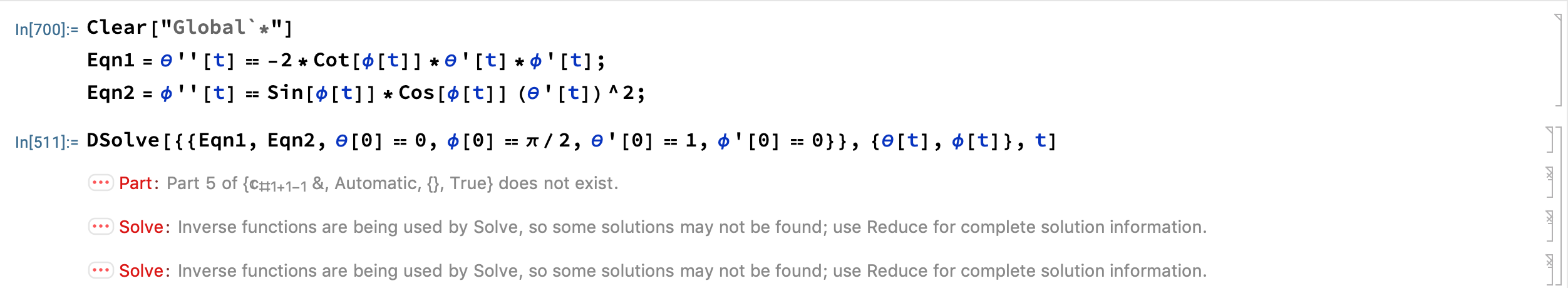
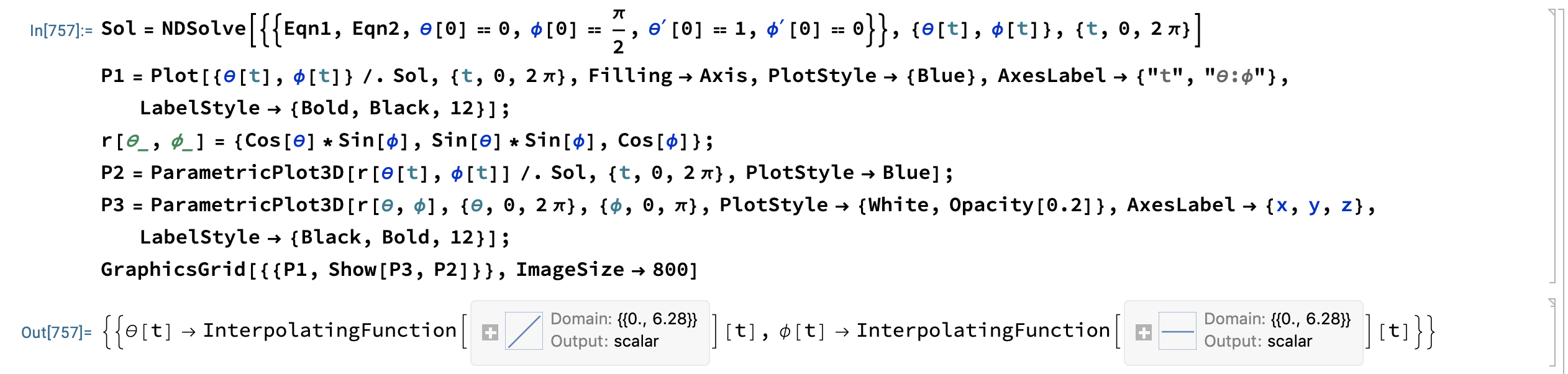
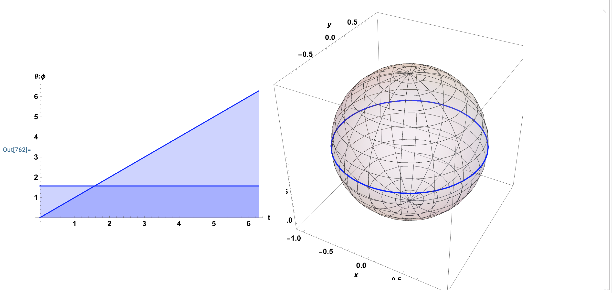
Figure 16: Even Computers Can Have Troubles: Despite having found and demonstrated (by hand) that the equator \((\theta(t),\phi(t))=(t,\pi/2)\) is a solution to the geodesic equations, Mathematica cannot find even this simply solution exactly via DSolve. It’s OK these equations are evidently hard to solve. However, solutions can be found using “numerical methods” NDSolve as seen in the plots.

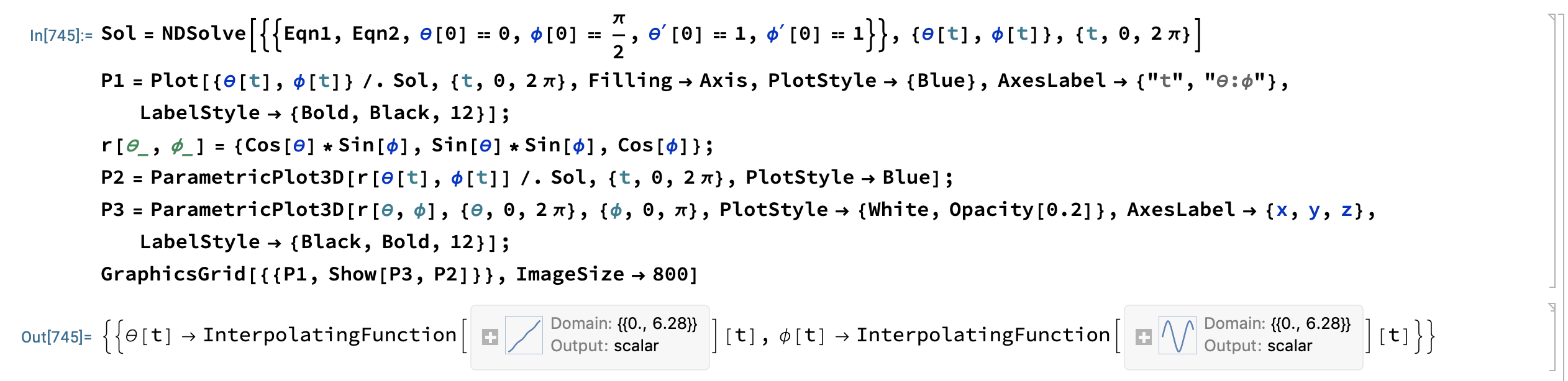
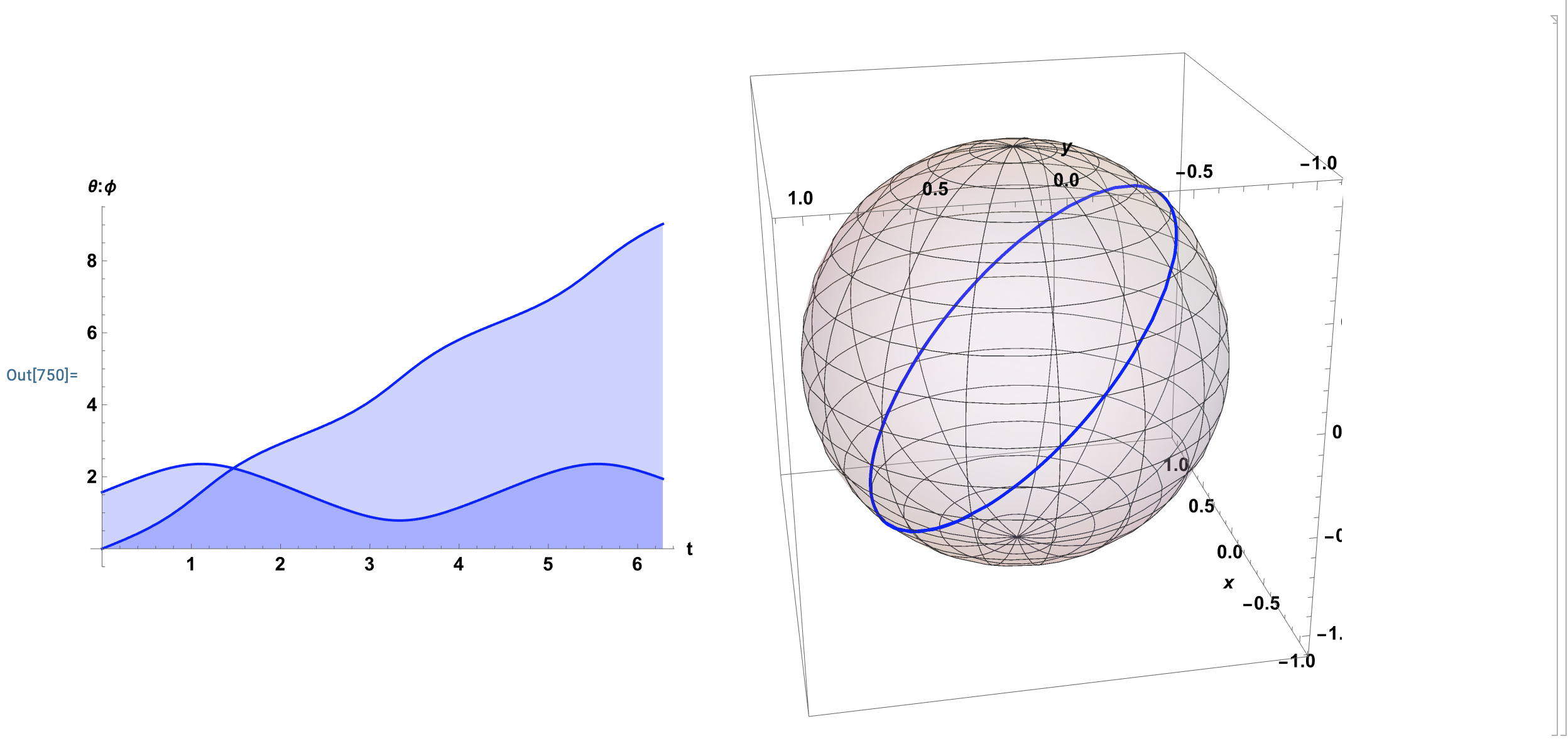
Figure 17: Guess and Check 1: Solution to the Geodesic Equations Seems to be a Great Circle.

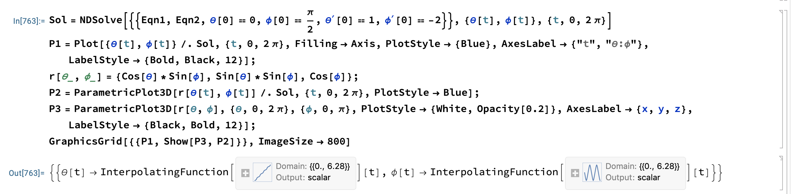
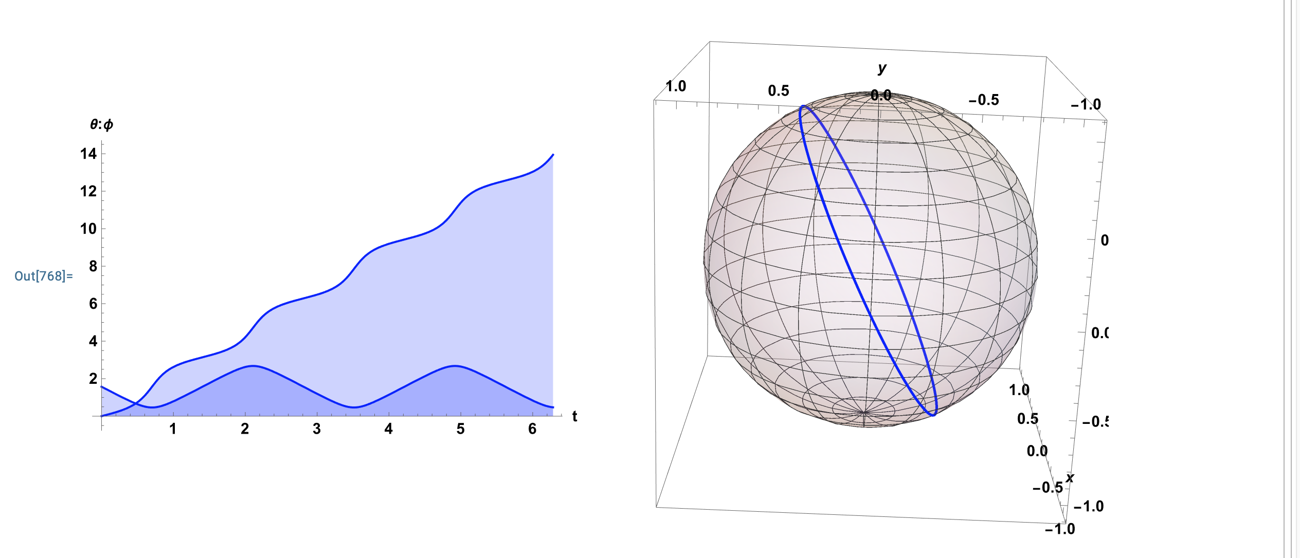
Figure 18: Guess and Check 2: Solution to the Geodesic Equations is Confirmed to be Great Circle.

Note: Showing the Great Circles are the only solutions to the geodesic equations on the sphere is possible using the qualitative solution methods of Clairaut and will be addressed in the “Additional Resources” section of this post.

Conclusion:

In this post we have tried to illustrate the interest Differential Geometers (those folks that like to mix Calculus with Geometry) have with the concept of curvature and geodesics. The technical and computational challenges are numerous in Differential Geometry. In this post we have illustrated a really interesting formula in Section The Big Result…A Euclidean Limit,

\[\begin{align} \Sigma_{i=1}^{3}\theta_{i}=\pi+\frac{A}{\rho^{2}}, \end{align}\]

that not only defines the curvature of a sphere but also in the same formula shows the implications of this definition (a two for one so to speak). Namely, curvature is that deviant quality inherent to a sphere which deforms the standard Euclidean result that angles of a triangle are required to add to \(180^{\circ}\). We have also seen that in defining the Differential Geometric equivalent of straight lines (the geodesics), the mathematical and computational complexity go up drastically. For example, it was necessary for us to work with higher dimensional arrays (i.e. beyond vectors and matrices) like the Christoffel Symbols \(\Gamma^{\sigma}_{\alpha\beta}\) and the Riemann Curvature Tensor \(R^{\sigma}_{\alpha\beta\kappa}\). To correctly handle computations involving these objects was a major reason I wrote the Maple package tensorAddOns. We will see more on tensors and usage of tensorAddOns package in future posts (see Figure 19).

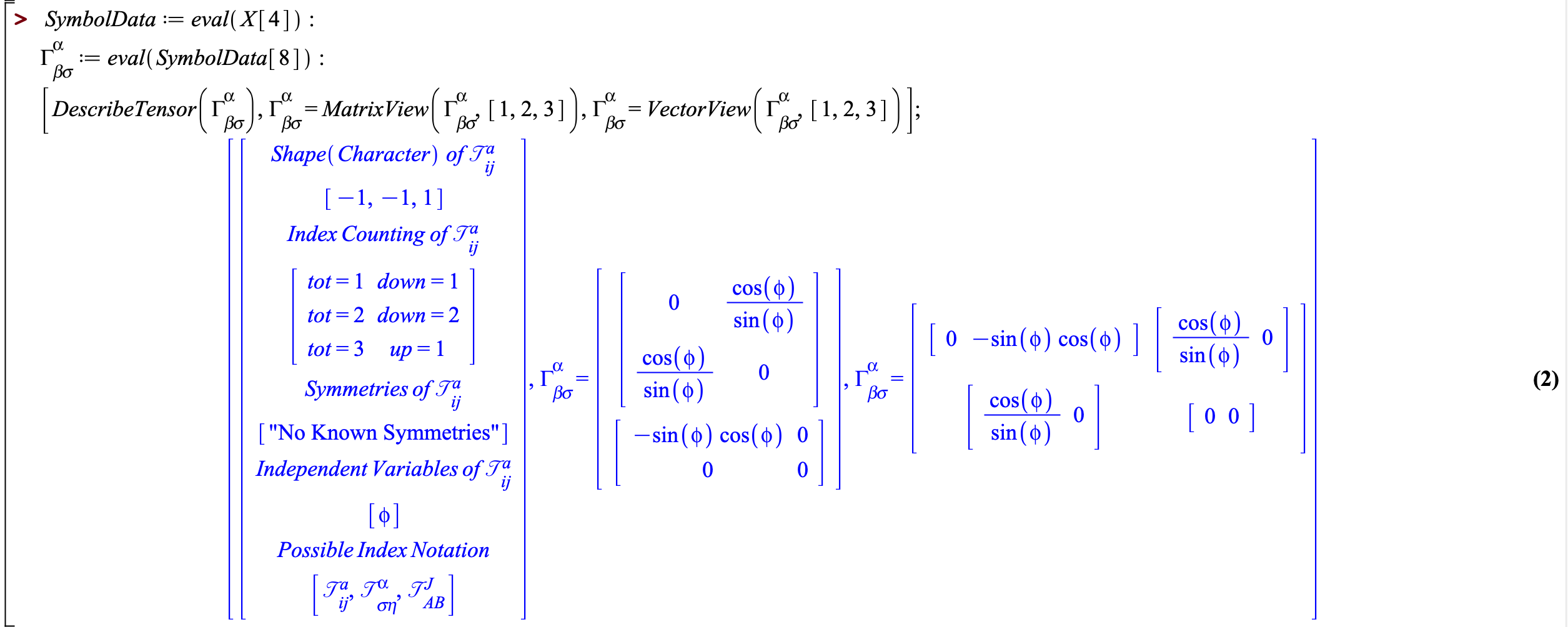
Figure 19: More tensors and the Maple tensorAddOns package to come in future posts.

Additional Resources Summary (link to Apple Books)

• Note: The formulas for Great Circles (in two parameterizations) between two points \(P=r(\theta,\phi)\) and \(Q=r(\Theta,\Phi)\) on a sphere is detailed in the “Additional Resources” section of this post.

• Note: The details behind using Stoke’s Theorem (three line integrals on the boundary curves) to evaluate the area of a geodesic triangle can be found in the “Additional Resources” section of this post.

• Note: Describing the Great Circles as solutions to the geodesic equations on the sphere is possible using the qualitative solution methods of Clairaut (i.e. a conservation law) and will be addressed in the “Additional Resources” section of this post.