Tensor Computations Using tensorAddOns

A demonstration and additional details behind the Maple package tensorAddOns. This is the companion file to the post Maple Conference 2022. In the near future, I will be writing more about tensors and tensor computations in Differential Geometry. The timing of the Maple Conference 2022 made this technical document necessary at this time, but more accessible posts will be coming soon. The mathematics software Maple, in particular the package I have written called tensorAddOns, will be key to correctly performing a wide variety of tensor computations in these upcoming posts.

Last Updated: Monday, October 31, 2022 - 17:04:53.

Motivation: On Matrices and Vectors as Examples of Tensors

An entry point to working with tensors (think, multidimensional data storage) is to be become familiar with matrices using kernel-index (or tensor) notation. Foreshadowing future posts related to tensors, here are some images that might begin to illustrate my thinking of vectors and matrices (examples of tensors) as storage mechanisms.

$Kernel-Index Notation for Vectors and Matrices. Index notation and the Einstein summation convention bring together components $D^{i},S_{j},M^{i}_{j}$ (objects to be stored) with their bases $e_{i},e^{j}, e^{j} \otimes e_{i}$ (storage space)$ $Kernel-Index Notation for Vectors and Matrices. Index notation and the Einstein summation convention bring together components $D^{i},S_{j},M^{i}_{j}$ (objects to be stored) with their bases $e_{i},e^{j}, e^{j} \otimes e_{i}$ (storage space)$

Figure 1: Kernel-Index Notation for Vectors and Matrices. Index notation and the Einstein summation convention bring together components $D^{i},S_{j},M^{i}_{j}$ (objects to be stored) with their bases $e_{i},e^{j}, e^{j} \otimes e_{i}$ (storage space)

Figure 2: Visual Summary of Kernel-Index Notation for Matrices

The Goal: In Code As On Paper

In the Section Motivation: On Matrices and Vectors as Examples of Tensors, matrices are alluded to as important pre-cursors to higher dimensional tensors. An important operation between matrices is matrix-matrix multiplication which has a higher dimensional equivalent between tensors called Transvection by Contraction (read, multiplication of tensors). In anticipation of multiplying tensors which will be greatly aided by the use of computational tools like Maple and tensorAddOns, we first do a proof-of-concept for matrix-matrix multiplication. In writing the tensorAddOns package it was very important to me that users work in code with tensors as they already know how to work with tensors on a sheet of paper.

(left) Matrix Multiplication in Tensor Notation (right) New tensorAddOns Functionality CreateTensor, DescribeTensor, and MatrixView (Note: prod is existing, but deprecated, functionality of the package tensor)

Figure 3: (left) Matrix Multiplication in Tensor Notation (right) New tensorAddOns Functionality CreateTensor, DescribeTensor, and MatrixView (Note: prod is existing, but deprecated, functionality of the package tensor)

What is… A Tensor and Tensor Multiplication?

It is helpful first to think of a tensor as a multidimensional storage mechanism for data of some kind. In the example below a tensor $T$ is a collection of patient medical data (name, height, and weight). There are a variety of ways to view this tensor $T^{a}_{bc}$ of 3D medical data in a human readable format using tensorAddOns[MatrixView]:

Figure 4: Think of a Tensor as a Storage Mechanism for Higher Dimensional Data

In Section The Goal: In Code As On Paper matrix-matrix muliplication is illustrated as transvection-by-contraction. The tensorAddOns package extends transvection/multiplication to tensors. For example, think of the data stored in the tensors $(A,B,V,W)$ below as simply the named location where some information could be written. Now let’s compute the product $A\cdot B \cdot V \cdot W$:

$Multiplication of the Tensors $A^{i}_{jk}$, $B^{n}_{m}$, $V_{p}$, and $W^{q}$ to get $(A\cdot B \cdot V \cdot W)_{m}=A^{i}_{jk}B^{j}_{m}V_{i}W^{k}$$

Figure 5: Multiplication of the Tensors $A^{i}_{jk}$, $B^{n}_{m}$, $V_{p}$, and $W^{q}$ to get $(A\cdot B \cdot V \cdot W)_{m}=A^{i}_{jk}B^{j}_{m}V_{i}W^{k}$

The Process and Philosophy: Maple Computations Then (Transport) Visualization

Tensors are used in many applications. For example, in Differential Geometry when computing the Parallel Transport Equations it is necessary to multiply a higher dimensional array (the Connection Coefficients) by a velocity vector. In this specific application and most likely any other application using tensors, it is incredibly important when computing multiplications to be sure the transvection by contraction is occuring on the correct indices. To ease the viewing and coding of these multiplicatons and to ensure the correctness of these computations was a primary goal in writing tensorAddOns.

The Process is to build on and work with Maple’s excellent (though, sadly, deprecated) tensor data type through new tensorAddOns functionality to maximize the chance of correctness of many tensor computations. Once these computations are complete, the function output can be passed to another application for solving (of ODEs, for example) and visualization (vector plots and animations, for example).

The Philosophy behind tensorAddOns is that

Users should work with tensors in code as they already know how to write tensors on a sheet of paper
Any input to a tensor functions calling sequence can be a symbol in tensor notation (via atomic variables). For example, when computing the Connection Coefficients, $\Gamma^{a}_{bc}$, in Differential Geometry via tensorAddOns[ConnectionCoefficients] it is known that a Metric Tensor, $g_{ab}$, is required and so the calling sequence should be something like tensorAddOns[ConnectionCoefficient]($g_{ab}$).
Any tensor functions output is nicely organized (but often long) summary viewable in a human readable format.
Any important or relevant computations used along the way in creating a tensor function summary should be accessible to the user. For example, upon passing $g_{ab}$ to tensorAddOns[ConnectionCoefficient] as an input to compute $\Gamma^{a}_{bc}$ it is necessary to perform a sub-computation $g_{\{ab,c\}}$, which is a complicated combination of partial derivatives of the metric tensor (sometimes called the Christoffel Symbols of the First Kind). A user can and should be able to access these Christoffel Symbols for later use and further manipulation.

The Process and Philosophy Put Into Practice. For example, in the Parallel Transport example below coordinates $q^{a}$ and a surface parametrization $\phi^{i}$ with respect to these coordinates are the inputs to a tensorAddOns function called TransportAndGeodesicEquationsOnSurface. The output of this function is summarized on screen (showing not only a view of the Christoffel Symbols, $\Gamma^{\sigma}_{\alpha\beta}$, but also the systems of ODEs representing both the Transport and Geodesic Equations). In the Accessible Data section of the output, we see that $\Gamma^{\sigma}_{\beta}$ has also been done as sub-computation which is the key matrix needed to build the Parallel Transport equations as a linear system of ODEs. This sub-computation can be accessed for export and then import to another program via MathML.

Figure 6: (left) Correct Maple Computations are the Most Important (right) Export Maple Output for Application and Visualization

Math Motivation and Coding Philosophy: From Gauss to Riemann Curvature

Recall from an earlier post Cascading Caveats that Gauss Curvature has been introduced as a “ratio of areas” in an “animated, graphic novel form” that the post Pattern Language and Storytime discusses might be a way to help make mathematics more accessible.

Figure 7: Gauss Curvature Illustration: A Ratio of Areas

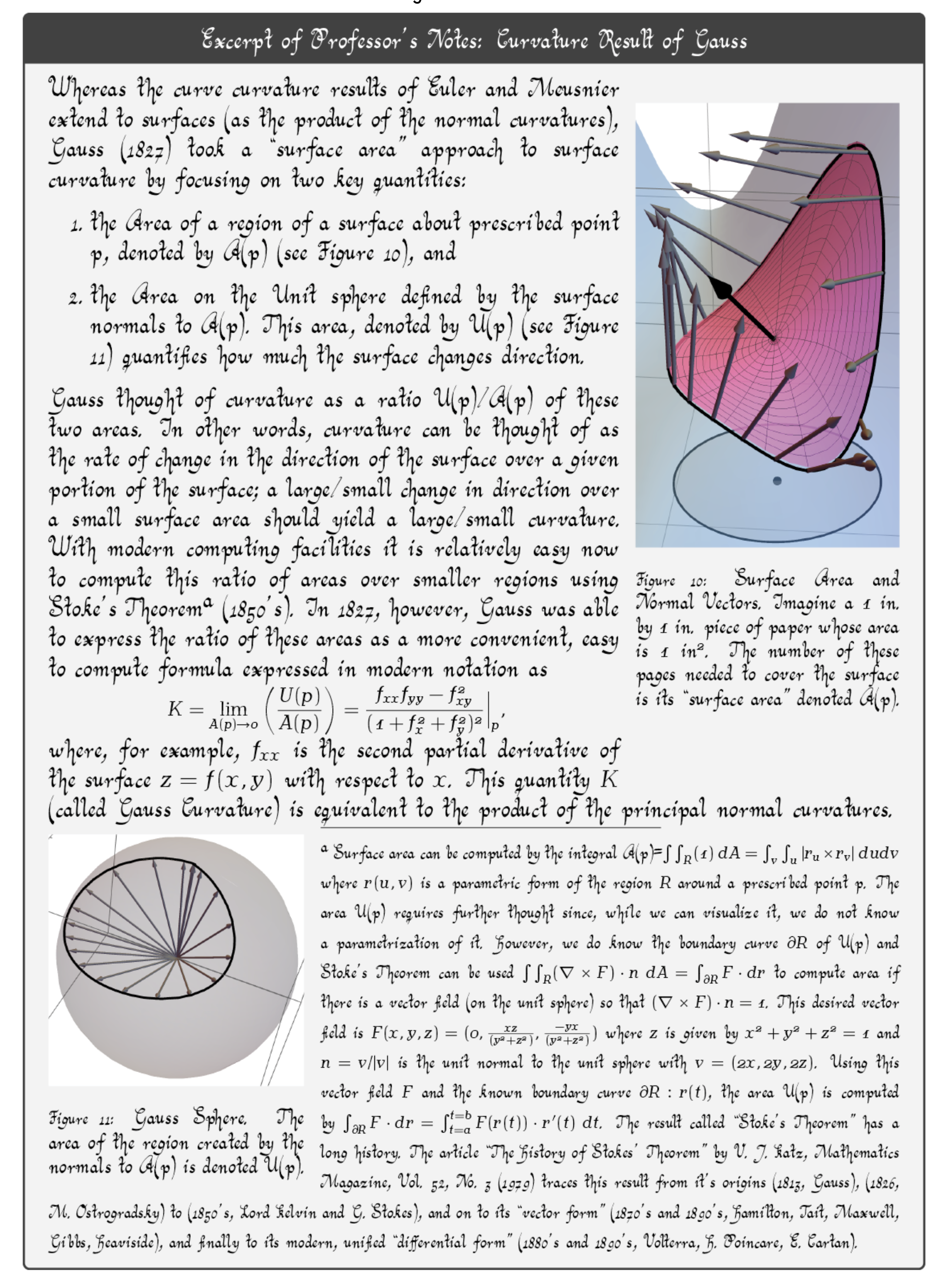
Gauss Curvature as an Animated Graphic Novel: Find “A Curvature Story” on Apple Books (shorturl.at/EGOXY)

Figure 8: Gauss Curvature as an Animated Graphic Novel: Find “A Curvature Story” on Apple Books (shorturl.at/EGOXY)

In this motivating example, we build on sections What is… A Tensor and Tensor Multiplication? and The Process and Philosophy: Maple Computations Then (Transport) Visualization to demonstrate the coding philosophy behind tensorAddOns by showing how tensorAddOns[RiemannCurvatureOnSurface] and tensorAddOns[SurfaceData] can be used to compute the Gauss Curvature from the Riemann Curvature.

Screenshots from tensorAddOns[RiemannCurvatureOnSurface] and tensorAddOns[SurfaceData] which Shows how the Riemann Curvature Defines the Gauss Curvature.

Figure 9: Screenshots from tensorAddOns[RiemannCurvatureOnSurface] and tensorAddOns[SurfaceData] which Shows how the Riemann Curvature Defines the Gauss Curvature.

A Comparison: The Packages tensorAddOns and Physics

Since deprecating the tensor package, Maple has given users the ability to work with tensors in two packages DifferentialGeometry and Physics. All I would really like to say here about the package DifferentialGeometry is that aspects of the design of the package tensorAddOns were to address some general shortcomings, as I saw them, behind the unintuitive input and output in say, for example, the setting up of Frames. On the plus side, both DifferentialGeometry and tensorAddOns can handle Connections in Anholonomic Frames.

Due perhaps to my penchant for kernel-index notation (tensor notation), I believe an example comparing tensorAddOns and Physics could be helpful.

Figure 10: A tensorAddOns vs. Physics package Comparison of the Computation of the Riemann Curvature Tensor of the Schwarzschild Metric

Technical Details: The tensor Data Type

Before we do an example that, arguably, only tensorAddOns might be able to do, let’s first take a look at the tensor data type that makes all of our tensor computation magic happen. What you will see in the first example is that, to Maple, the tensor data type is a table which is first and foremost comprised of

it’s shape or index character (index_char),
components (compts).

The tensor data type (specifically, it components) are further comprised of

symmetries (as an aspect of it’s components).

The tensorAddOns package (specifically the function CreateTensor) extends the tensor package functionality (specifically the function create) with regards to these tensor symmetries. As addressed in the second example, there are many additional symmetries that can be applied to a tensor once it has been created via the function AssignIndexingSymmetry.

Figure 11: Technical Details of tensor Data Type

Figure 12: Technical Details of tensor Data Type

The Question: An Example Only tensorAddOns Can Do?

In conclusion, we show an example that, because of it’s anholonomic nature, makes us wonder if the tensorAddOns package in Maple is the only program written that can do it? We welcome your feedback.

Figure 13: tensorAddOns Computes the Riemann and Ricci Curvature Tensors in an Orthonormal, Anholonomic Frame

More Info: Check out our blog unconcisemath.com

Currently 36 functions in the package tensorAddOnsTools and tensorAddOnsComps.
Many documentation examples have been written that are in need of testing and demonstration.

Figure 14: See the post Maple Conference 2022 on our blog unconcisemath.com.